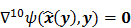
Impact Factor
- Issue 14; 2026
- Issue 13; 2026
- Issue 12; 2026
- Issue 11; 2026
- Issue 10; 2026
- Volume 16; 2026
- Advance Articles
- Past Issues
- Cover Images
- Cover Suggestion
- Index & Coverage
- Special Issues
Introduction
Background
Statistical Analysis Techniques
Applications
Discussion
Acknowledgements
References
International Journal of Biological Sciences
International Journal of Medical Sciences
 Global reach, higher impact

Theranostics 2013; 3(10):741-756. doi:10.7150/thno.6815 This issue Cite
Review
Quantitative Statistical Methods for Image Quality Assessment
Joyita Dutta1, Sangtae Ahn2, Quanzheng Li1 ![]()
1. Center for Advanced Medical Imaging Sciences, Harvard Medical School, Massachusetts General Hospital, Boston, MA, USA;
2. GE Global Research Center, Niskayuna, NY, USA.
Received 2013-6-1; Accepted 2013-7-19; Published 2013-10-4
Abstract
Quantitative measures of image quality and reliability are critical for both qualitative interpretation and quantitative analysis of medical images. While, in theory, it is possible to analyze reconstructed images by means of Monte Carlo simulations using a large number of noise realizations, the associated computational burden makes this approach impractical. Additionally, this approach is less meaningful in clinical scenarios, where multiple noise realizations are generally unavailable. The practical alternative is to compute closed-form analytical expressions for image quality measures. The objective of this paper is to review statistical analysis techniques that enable us to compute two key metrics: resolution (determined from the local impulse response) and covariance. The underlying methods include fixed-point approaches, which compute these metrics at a fixed point (the unique and stable solution) independent of the iterative algorithm employed, and iteration-based approaches, which yield results that are dependent on the algorithm, initialization, and number of iterations. We also explore extensions of some of these methods to a range of special contexts, including dynamic and motion-compensated image reconstruction. While most of the discussed techniques were developed for emission tomography, the general methods are extensible to other imaging modalities as well. In addition to enabling image characterization, these analysis techniques allow us to control and enhance imaging system performance. We review practical applications where performance improvement is achieved by applying these ideas to the contexts of both hardware (optimizing scanner design) and image reconstruction (designing regularization functions that produce uniform resolution or maximize task-specific figures of merit).
Keywords: tomography, image quality metrics, local impulse response, resolution, variance.
Introduction
Medical image reconstruction methods seek to estimate images representing some physical signal in the 3D or 2D spatial domain from data belonging to a different physical domain of observation. Since these estimates are functions of noisy data, there is some inherent uncertainty in them. Apart from the noisy data, the final reconstructed image quality also depends on parameters associated with the system model and the reconstruction method. Commercial imaging systems usually generate only the reconstructed images without providing quantitative metrics representing their quality and reliability. These metrics, which can facilitate both qualitative interpretation and quantitative analysis, are just as critical as the actual image estimate. In view of the paramount importance of quantitative image quality measures, this review surveys a range of techniques to compute such metrics for reconstructed images. While the primary emphasis here is on emission tomography, including positron emission tomography (PET) and single photon emission computed tomography (SPECT), we will discuss parallel efforts in computed tomography (CT) and magnetic resonance imaging (MRI). For the reader's convenience, an alphabetical list of the acronyms used in the text is provided in Table 1.
List of abbreviations.
| Acronym | Expanded form |
|---|---|
| CHO | Channelized Hotelling observer |
| CNR | Contrast-to-noise ratio |
| CRC | Contrast recovery coefficient |
| CRLB | Cramér-Rao lower bound |
| CT | Computed tomography |
| EM | Expectation maximization |
| EMSE | Ensemble mean squared error |
| FWHM | Full width at half maximum |
| ICA | Iterative coordinate ascent |
| LIR | Local impulse response |
| LPR | Local perturbation response |
| LS | Least squares |
| MAP | Maximum a posteriori |
| MAPEM | Maximum a posteriori expectation maximization |
| MCIR | Motion-compensated image reconstruction |
| ML | Maximum likelihood |
| MLEM | Maximum likelihood expectation maximization |
| MR | Magnetic resonance |
| MRI | Magnetic resonance imaging |
| NPW | Non-prewhitening |
| OSEM | Ordered subsets expectation maximization |
| OSL | One-step-late |
| PCG | Preconditioned conjugate gradient |
| PET | Positron emission tomography |
| PSF | Point spread function |
| QPLS | Quadratically penalized least squares |
| ROC | Receiver operating characteristic |
| ROI | Region of interest |
| SNR | Signal-to-noise ratio |
| SPECT | Single photon emission computed tomography |
| UQP | Uniform quadratic penalty |
| WLS | Weighted least squares |
Reconstruction methods fall into two main categories: analytical techniques and model-based iterative techniques. Analytical approaches offer a direct, closed-form solution to estimate the unknown image. In comparison, model-based iterative approaches use numerical techniques to generate an image that can be deemed as the “best” choice in terms of some suitable figure of merit. These methods, while slower and more complex, generate enhanced image quality [1] through improved modeling of both the physical processes that yield the measured data and the statistical noise therein. For linear analytical approaches such as filtered backprojection [2], it is relatively straightforward to characterize reconstructed image noise and to compute closed-form expressions for image quality metrics [3,4]. The task is far more involved for iterative methods that incorporate more complex nonlinear formulations. Iterative approaches have become ubiquitous in PET and SPECT, for which these methods have been shown to offer tremendous image quality improvement relative to analytical methods. While analytical methods continue to dominate the CT and MR arenas, iterative methods are steadily gaining popularity for applications such as low-dose CT and fast MRI, where the margin of image quality improvement these methods yield relative to analytical methods is more significant. Multiple strategies for characterizing iteratively reconstructed images have emerged in the recent past.
In the absence of closed-form expressions, quality measures for reconstructed images can be computed using a Monte Carlo approach, which generates sample means derived from a large number of noise realizations of the data. However, the utility of this brute force approach is limited due to the presence of tuning parameters associated with iterative reconstruction schemes. Examples of these tuning parameters include the cutoff frequency of the filter in filtered backprojection, the stopping criterion for methods belonging to the expectation-maximization (EM) family, and the regularization parameter for maximum a posteriori (MAP) estimation. The choice of these parameters influences the properties of the final reconstructed image and hence also the values of the image quality metrics. Complete characterization of reconstruction approaches would entail repeated computation of these metrics for multiple choices of the tuning parameters, which is a prohibitively expensive proposition. Furthermore, in clinical applications, usually only one data set is available. As a result, techniques that compute image quality metrics from multiple noise realizations have limited clinical utility.
To circumvent this problem, multiple approaches presenting approximate closed-form expressions for different metrics have emerged over the last two decades. These fall under two major categories: fixed-point and iteration-based analysis. The first category assumes that the iterative algorithm used for reconstruction has converged at a unique and stable solution allowing us to compute image statistics, independent of the iteration number. This is applicable to gradient and preconditioned gradient based algorithms when used to optimize well-behaved objective functions [5,6,7]. Numerical optimization algorithms, if iterated until convergence, matter only when it comes to computational cost, in terms of reconstruction time and memory usage. If, however, an algorithm is terminated before convergence, the iteration number affects the final image quality. In certain cases, early termination is an accepted way to control the noise in the reconstructed image. For example, in clinical PET imaging, it is a common practice to stop the OSEM (ordered subsets expectation maximization) algorithm after only a few iterations, before the images become unacceptably noisy. The second category of noise analysis techniques, therefore, focuses on algorithms which either are terminated before convergence to control the noise in the final reconstructed images [8,9] or fail to converge to a unique and stable solution [10,11]. The statistics computed for these methods, therefore, are functions of iteration number [12,13,14]. In this paper, we will review established image reconstruction schemes, describe some key mathematical techniques developed for analyzing reconstructed images, explore extensions of some of these methods to a range of contexts (including nonquadratic penalties, dynamic imaging, and motion compensation), and finally discuss ways to utilize our knowledge of image statistics to enhance image quality either by optimizing regularization or by optimizing instrumentation.
Background
Iterative Reconstruction Approaches
Throughout this paper, the 3D (or 2D) unknown image is discretized and represented by a 3D (or 2D) array of voxels (or pixels), which is then lexicographically reordered and denoted by a column vector  . Boldface notation is used to distinguish a vector quantity from a scalar. The physical connotation of this unknown image depends on the imaging modality in question. For PET and SPECT, it is the spatial distribution of a radiotracer. For CT, it is a spatial map of attenuation coefficients. For MRI, it is a spatial map of transverse magnetization resulting from the interplay between radiofrequency signals and hydrogen nuclei in tissue in the presence of a strong DC magnetic field. The data is represented by another column vector
  . For PET, SPECT, and CT, the data vector is a lexicographically reordered version of projection data. For MRI, the data vector consists of sample points in k-space, which is the spatial Fourier transform of the unknown image. All model-based reconstruction schemes rely on a forward model that maps the image space to the data space. In other words, for a given image
  , the forward model predicts a data vector
  as a function of the image. When the mapping from the image domain to the data domain is a linear transformation (as is the case in PET, SPECT, CT, and MRI), the forward model can be described using a matrix
  such that
  . The reconstruction routine seeks to solve the corresponding inverse problem of determining an estimate,
  , of the unknown image as some explicit or implicit function of the observed noisy data, say
  .
.
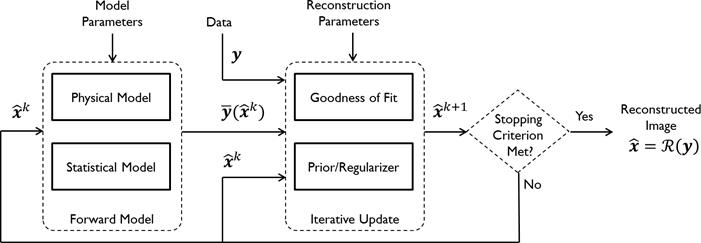
Figure 1 summarizes the model-based iterative reconstruction procedure. All model-based iterative reconstruction methods begin with an initial estimate  of the unknown image and update this estimate based on the similarity (or difference) between the data predicted by the forward model,
  , and the measured data,
  , and on any prior knowledge one might have about the image. This procedure is repeated or “iterated” generating a sequence of successive estimates
  till some stopping criterion is satisfied. Iterative reconstruction techniques have two key components, an objective function and an optimization algorithm, as described below:
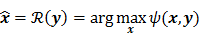
Schematic illustrating the model-based iterative reconstruction procedure. The forward model predicts the data,  , as a function of the image
  . The reconstruction routine seeks to determine the unknown image as some explicit or implicit function,
  , of the data. For iterative reconstruction, this function is an implicit function given by the maximum of some objective function:
 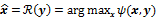 . The objective function,
  , depends on both the goodness of fit between the predicted and measured data and on prior information about the unknown image. At the end of each iteration, the current image
  is replaced by an updated estimate
  until some stopping criterion is reached.
I. Objective Function
The objective function (or the cost function) is a figure of merit for image reconstruction. The final reconstructed image should maximize (or minimize) this figure of merit. The chief constituent of the objective function is a data fidelity or goodness of fit term, which quantifies the discrepancy between the measured data and the predicted data. The sum of squared residuals, 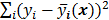 , and the weighted sum,
 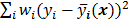 , are examples of the goodness of fit used in the ordinary least squares (LS) and weighted least squares (WLS) techniques respectively. Alternatively, if the measured data
  is modeled as a random vector with a conditional probability density function
  , then the likelihood
  or the log likelihood
  can be used as a measure of the goodness of fit. This is the basis for likelihood-based reconstruction methods, including maximum likelihood (ML). From this statistical perspective, the forward model
  represents
  , the mean or expectation of the data vector conditioned on (and hence parameterized by) the given image,
  . The two most widely used probability distributions in medical imaging are the Gaussian and Poisson distributions. If the data is contaminated with independent identically distributed Gaussian noise, then the log likelihood reduces to a negative LS formulation,
  . If the Gaussian noise is independent but heteroscedastic, that is,
 for
for  , then the log likelihood leads to the negative WLS formulation,
  where
where  . If the data
  are independent Poisson random variables whose means are
  , then the log likelihood can be written as
 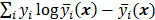 . This Poisson likelihood model is widely used in PET and SPECT.
Most medical imaging inverse problems are ill-conditioned. This means a large change (usually in the higher spatial frequency components) in the image  may elicit only a small change in the data
  . Such small changes may be virtually indistinguishable from noise. In such cases, attempts to maximize the goodness of fit by enforcing strict agreement with the noisy data may cause noise amplification in the reconstructed images, a phenomenon known as overfitting. This is a commonly acknowledged problem with the ML image estimate in emission tomography. Two common approaches used to alleviate this problem are early termination and regularization. Post-reconstruction filtering, in combination with early termination, is also frequently used [15]. Early termination will be discussed subsequently in the context of the EM family of optimization algorithms. Regularization techniques augment the objective function by a regularizer function, which serves to encourage or penalize certain characteristics in
  , based solely on prior knowledge and not on the data. This leads to the class of methods referred to as maximum a posteriori (MAP) or penalized maximum likelihood in medical imaging literature. From an algebraic perspective, this function could be viewed as a penalty function that constrains the search space based on additional knowledge concerning the nature of the solution and thereby facilitates convergence and eases the task for the optimization algorithm. From a statistical perspective, this function could be viewed as a prior probability distribution for the random vector
  . In essence, the reconstructed image should now maximize the posterior probability, given by
 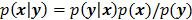 , or, more commonly, its logarithm. The relative contributions of the data-fitting and regularization components of the resulting objective function are determined by a tuning parameter usually referred to as a regularization parameter or a hyperparameter. Quantitative metrics for reconstructed image quality are functions of this parameter.
II. Optimization Algorithm
The numerical optimization algorithm is a recipe which generates the image that maximizes the selected objective function. An iterative algorithm may not be required if a closed-form solution to the inverse problem exists or, in other words, if  is an explicit function. However, this is not the case for the highly nonlinear Poisson likelihood function. Also, even when closed-form solutions exist, they often require a matrix inversion step that carries a large computation cost. Therefore, an iterative algorithm is usually the ultimate resort for most large-scale real-world problems. Consequently, state-of-the-art PET and SPECT reconstruction methods are iterative in nature. The expectation maximization (EM) family [8,9] represents a popular class of iterative algorithms. The EM algorithm, developed as a numerical tool for ML estimation [16], is based on the notion of unobservable data. This algorithm iterates by alternating between an expectation (E) step and a maximization (M) step. The E-step computes the expectation of the complete-data log likelihood function conditioned on the current estimate of the image,
  , and observed data,
  ; this is equivalent to calculating the mean of the unobserved (latent) variables conditioned on the current estimate and observed data when the complete-data probability distribution is from an exponential family. The M-step computes the unknown image,
  , which maximizes this log likelihood function. While MLEM, in theory, should ultimately converge to the ML estimate, its convergence is slow for the Poisson likelihood [17]. The ordered subsets EM (OSEM) method [10] is a modification of the EM algorithm which divides the data into a number of groups and bases each update on only the subset of data belonging to one group at a time. OSEM is the current standard for clinical PET and SPECT scanners since this technique and its variants [11,18,19] significantly accelerate convergence rate. However, its major limitation is that it does not converge to a stable solution. Due to the absence of a regularization term, MLEM and its OS version typically produce high noise levels for a large number of iterations. The general practice, therefore, is to terminate these methods early to limit noise amplification caused by overfitting [20,21]. When early termination is exercised, the final image depends on the initial image,
  , the algorithmic details, and the final iteration number. The statistical properties of this final image must therefore be derived as function of these quantities. This leads us to what is referred to as iteration-based analysis in this paper.
A variety of generic gradient-based optimization schemes have also been used to maximize the MAP objective function. Specifically, the preconditioned conjugate gradient (PCG) [5,6,7] and iterative coordinate ascent (ICA) [22,23] algorithms have been shown to yield speedy convergence. Unlike the ML case, the inverse problem for the MAP objective function is less ill-conditioned and, hence, more well-behaved. For a large enough regularization parameter, these algorithms can actually be iterated to convergence without the previously mentioned noise amplification and overfitting problems. The advantage of this approach is that, as long as an algorithm is globally convergent, i.e., it converges to a fixed point regardless of initialization, the final reconstructed image is independent of the initial image, the iteration number, the algorithm type, and algorithmic parameters, such as the step size. In this case, it is sufficient to characterize the statistical properties at the point of convergence, leading to fixed-point analysis methods. While the point of convergence is independent of the algorithm, it continues to depend on the objective function and, therefore, on the choice of the regularization parameter.
Image Quality Measures
The choice of statistical measures of image quality depends on the goal of the imaging procedure. If the sole objective is to tell whether a cancerous lesion is present or absent in the image, the task at hand is a statistical detection task. In contrast, a variety of oncological and pharmacokinetic studies seek to quantify the tracer uptake in each voxel or inside a region of interest spanning several voxels. From a statistical perspective, this is an estimation task. Computing image quality measures for a given image reconstruction scheme then boils down to characterizing the underlying statistical estimation scheme. The Cramér-Rao lower bound (CRLB) offers one way to characterize an estimator. Hero et al. [24] examined delta-sigma tradeoff curves (plots of the bias gradient norm  against the standard deviation
  ) that were generated using the uniform CRLB. Meng and Clinthorne [25] extended this approach to derive a modified uniform CRLB, which they used to characterize SPECT scanner designs in terms of achievable resolution and variance. While CRLB-based approaches are significant, in this paper, we focus on an alternative (and more popular) class of techniques which seek to characterize reconstruction methods using resolution and covariance measures, as described below:
I. Covariance
For any image reconstruction method, the estimated image  is some explicit or implicit function,
  , of the noisy data
  . By virtue of this functional dependence, if
  is a random vector with a probability density function
  , parameterized by the true image
  ,
,  should also be a random vector with a probability density function parameterized by
  . Noise in the reconstructed images can therefore be characterized by the covariance matrix
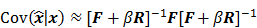
  . The diagonal elements of this matrix represent the ensemble variance at each voxel of the reconstructed image, while the off-diagonal elements represent the correlation between the voxels when they are normalized. As an example, let us consider the quadratically penalized least squares objective function (QPLS), which is obtained by augmenting the LS objective function,
  , by a quadratic regularization term of the form
  . When no nonnegativity constraint is imposed, the reconstruction operator ℛ for the QPLS objective function is linear. If the data noise is additive white Gaussian, then the covariance matrix
  of the reconstructed image is independent of the true image
  . However, this does not apply to more general cases. When the data noise is Poisson distributed (as is the case in emission and transmission tomography),
  has a strong dependence on
  . We will survey a range of noise analysis techniques that derive approximate closed-form expressions for
  addressing its dependence on the true image
  .
.
II. Resolution
It is customary to assess estimators in terms of the inherent tradeoff between their bias and variance. Regularized reconstruction techniques reduce image variance at the cost of added image bias. For smoothing regularizers, this bias largely manifests as a spatial blur or, in other words, as a reduction in image resolution. Image resolution is a quantitative measure that characterizes the degree of blurring a sharp structure (such as a spatial impulse function) undergoes and is dependent on both the physical and the statistical model of the system and on any tuning parameters associated with the reconstruction method. Even for unregularized objective functions, early termination of the optimization algorithm could produce bias. When initialized by a uniform intensity image, as is the usual case with OSEM reconstruction of clinical PET images, early termination tends to bias the image toward uniformity causing a spatial blur. It is therefore widely accepted to assess image reconstruction methods by their resolution-covariance characteristics as a surrogate for their bias-variance characteristics. Thus, along with image covariance, image resolution is a critical image quality measure.
Linear shift-invariant systems produce a blurring effect that is independent of voxel location. The resolution for such systems can be determined from a global impulse response or a point spread function (PSF), which is the result obtained when the original image is an impulse function in space. This measure is useful for linear analytical reconstruction approaches, such as filtered backprojection. For model-based iterative reconstruction methods that are nonlinear, the resolution of the reconstructed images is spatially varying and can depend on the true image. To quantify the resolution properties for such cases, one can analyze the local impulse response (LIR) [26,27] at a given voxel i, which can be computed as:

where  denotes a unit impulse at voxel
  , or, in other words, an image vector with a value of one at the
  th spatial location and zeros elsewhere. The LIR measures the change in the mean reconstructed image caused by an infinitesimal perturbation at a particular location (voxel
  ) in the true image
  . The location dependence of this metric ensures that it captures the spatially varying nature of a nonlinear estimation technique. The dependence of the LIR on the true image ensures that it captures the object dependent nature of a nonlinear estimation technique.
Statistical Analysis Techniques
Fixed-Point Analysis
In this section, we will outline some methods to compute approximate closed-form expressions for the covariance and local impulse response of reconstruction methods that converge at a unique and stable fixed point. These fixed-point methods can be based on either discrete space or continuous space approaches. Both approaches are popular and have been adapted for a range of specialized imaging applications encompassing different imaging modalities.
I. Discrete Space Methods
For ML and MAP estimates based on the Poisson likelihood, explicit analytical functional forms are unavailable. Instead, these estimators are implicit functions of the data  defined as the maximum of some objective function,
  :
:
While a closed-form expression for  may not exist, Fessler [28] showed that approximate expressions for the mean and covariance of
  can be obtained utilizing Taylor series truncation along with the chain rule of differentiation. The necessary condition for optimality requires that this maximum correspond to a stationary point, defined as a point where the gradient with respect to
  is the zero vector. Stated in mathematical notation, this means:
Here  represents the column gradient operator with respect to the first argument of the function
  . By using a first order Taylor series approximation centered at the mean data
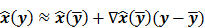
  , this implicit function can be approximated as:
where  denotes the Jacobian matrix (the matrix of all the first-order partial derivatives). The corresponding approximation for the covariance is:

where  represents the matrix or vector transpose. Even though
  is unknown,
  can be approximately computed by applying the chain rule of differentiation to the stationarity condition, yielding:

where  denotes the Hessian of
  with respect to the first argument and
  represents a composition of the column gradient operator with respect to the first argument and the row gradient operator with respect to the second argument. The covariance can then be computed in closed form as:

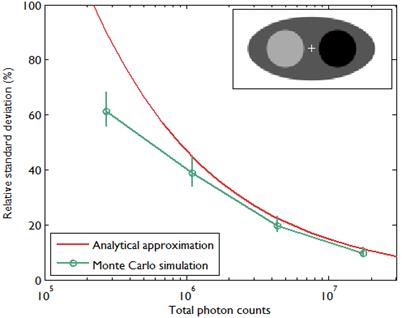
A comparison between the covariance predicted by the above approach and that obtained using Monte Carlo simulations is shown in Figure 2, which presents the results of a 2D simulation study similar to that shown in Figure 7 of [28]. This study demonstrates that the analytical and Monte Carlo approaches exhibit good agreement for data with high counts (i.e., low noise). The corresponding variance images are shown in Figure 3.
Comparison of predicted standard deviation from an analytical expression given in [28] and sample standard deviation calculated from Monte Carlo simulations as in Figure 7 of [28]. The standard deviation was calculated at the central pixel indicated by a (+) symbol inside the 2D digital phantom image in the inset. The image size was 128 by 64 pixels with pixel size 4.5 mm, and the sinogram size was 192 radial bins by 96 angular bins with a radial bin spacing of 4.5 mm. The emission activity was 3 in the hot region (black), 2 in the background (dark gray), and 1 in the cold region (light gray). The attenuation coefficient was 0.013/mm in the hot region, 0.0096/mm in the background, and 0.003/mm in the cold region. The simulated photon counts were 0.25M, 1M, 4M, and 16M. The background events such as randoms and scatter were simulated as a uniform field with 10% of true events. For each photon count, 100 data sets contaminated by Poisson noise were generated. For each data set, a quadratically penalized likelihood image was reconstructed using 20 iterations of an ordered subset version of De Pierro's modified EM [29] with 8 subsets. The regularization parameter was chosen to be proportional to the total count as in [28]. The standard errors of the standard deviation were computed by bootstrapping.
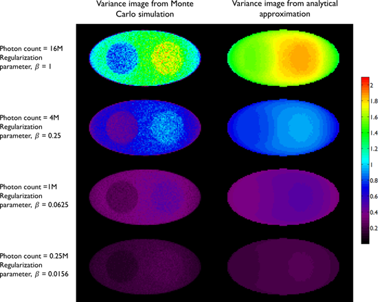
Variance images from the simulation study in Figure 2. The left column shows empirical estimates obtained from Monte Carlo simulations with 100 noise realizations. The right column shows the predicted variance from a single noise realization using the analytical approach in [28]. The rows correspond to the following photon count/regularization parameter combinations: 0.25M/0.0156, 1M/0.0625, 4M/0.25, 16M/1.
Fessler [28] also provided a second-order Taylor series approximation for the mean of the unknown estimator,  , which can be used to analyze the bias and resolution. However, unlike the covariance, the approximation for
  cannot be written in a simple matrix form. Its utility is therefore limited to applications involving fewer parameters. A less accurate but more tractable alternative widely used in literature is a zeroth order approximation for the mean,
  . In this approximation, the ensemble mean of an estimator is approximated by the noiseless estimate.
These mean and covariance computation methods preclude inequality constraints and stopping rules (for early termination). Fortunately, since nonnegativity constraints have minimal influence on the nonzero voxel intensities, mean and variance values for unconstrained and constrained estimators are approximately equal for high intensity regions [30]. An approach that accounts for the effect of the nonnegativity constraint on the variance using a truncated Gaussian model can be found in [31].
To study the resolution properties of  , Fessler and Rogers [27] derived approximate expressions for the linearized LIR by applying a technique based on Taylor series truncation around
  and the chain rule of differentiation, similar to that used for the covariance approximation:

Consider the penalized likelihood objective for emission tomography:
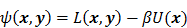
Here  represents the Poisson log likelihood function,
  is the regularization parameter, and
 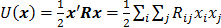 is a quadratic penalty function, where the matrix
  is the Hessian for
  . Since most medical images of interest tend to be spatially smooth, the quadratic penalty function is set to compute the sum of squared intensity differences between neighboring voxel pairs in the image
  :
:
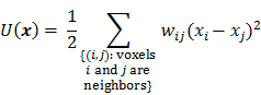
where  is a nonnegative weight. Usually
  is chosen to be inversely proportional to the distance between voxels
  and
and  . In this case, the elements of the matrix
  are given by
  and
and  when voxels
  and
and  are neighbors and
  otherwise. This penalty function with spatially invariant weights
  , in common parlance, is referred to as the uniform quadratic penalty (UQP). Penalization of quadratic differences in intensity essentially enforces spatial smoothness in the reconstructed image. From a statistical perspective, this class of penalty functions corresponds to a Gaussian prior probability distribution. Quadratic penalties are relatively straightforward to analyze since they have a constant second derivative and therefore remain exact under the Taylor series truncation procedure described earlier. Adapting the linearized LIR to this estimation problem, Fessler and Rogers [27] derived a fundamental result for emission tomography. They demonstrated that standard spatially invariant regularizing functions, such as the UQP, produce spatially varying resolution in the reconstructed image. This is a key observation since the nonuniformity of spatial resolution in the images directly impacts their quantitative interpretation. As an example of the effect of nonuniform spatial resolution, consider a scenario where a reconstructed PET image shows two lesions at two locations with two different local full widths at half maximum (FWHMs). At the location where the FWHM is higher (resolution is poorer), the lesion will be smeared over several voxels yielding a smaller value for radiotracer uptake than that observed for the location with lower FWHM (higher resolution). The lesion at the first location will therefore appear less threatening than it actually is.
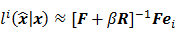
For the quadratically penalized objective, the local impulse response and covariance can be approximated as:


where  is the Fisher information matrix for the Poisson likelihood model and
  is a unit impulse at voxel
  . These equations, which are a direct outcome of the methods in [27] and [28], involve prohibitively expensive matrix operations and therefore are not practical for standard-sized 3D medical images. In light of their intractability, these expressions were further simplified by Qi and Leahy [32,31] using a Fourier domain approach [33] yielding the following closed-form expressions for the local impulse response and variance:
,

where  represents the
  th column of the covariance matrix
  ,
,  and
and  represent the Kronecker forms of the 3D Fourier transform and 3D inverse Fourier transform respectively,
  represents the 3D Fourier transform of the
  th column of a scaled, approximate data-independent version of
  ,
,  represents the 3D Fourier transform of the
  th column of
  , and
, and  , referred to as an aggregate certainty measure [27], is computed such that
  is an approximation for the
  th diagonal element of
  . A method to accurately estimate the certainty measure from noisy data particularly for very low counts can be found in [34]. To facilitate interpretation, one could resort to scalar measures derived from the above expressions. Since it may be tedious to compute the full covariance matrix, one option is to focus on its diagonal which represents individual voxel-wise variances. Instead of computing the LIR for each voxel, one could look at the LIR contrast recovery coefficient (CRC), which is defined as the peak of the LIR [31,32]. The CRC is an accepted alternative to the FWHM as a measure of resolution. Simplified expressions for both of these quantities are provided in [31].
II. Continuous Space Methods
Discrete space approaches, though reasonably accurate, are computationally expensive, since they typically require the inversion of large Hessian matrices. Even with Fourier-based approaches that use circulant approximations for the Hessian matrices, these methods are computationally demanding. Fessler [35] developed a faster alternative which replaces the usual discrete system model with locally shift-invariant, continuous space approximations. This approach starts with a discrete formulation, switches to the continuous domain for some intermediate steps, and then reverts back to the discrete domain. The underlying approximate expressions for the LIR and covariance are the same as those used for discrete space fixed-point analysis:
But in order to avoid expensive matrix manipulations, the matrices  and
and  are replaced by continuous space operators. The approximation for
  is based on the Radon transform, a view-independent, radially shift-invariant blur, and an analytical measure of the effective certainty for a given voxel and a given detector angle or line of response. The approximation for
  is based on the continuous space representation of the quadratic penalty,
  where
where  is a continuous space version of the image. Although the accuracy of continuous space methods is limited by the simplistic nature of the system model used, they are useful because of their speed. These methods have been applied to both 2D and 3D CT and PET [36,37,38].
III. Nonquadratic Regularizers
One limitation of quadratic penalties is that they tend to oversmooth edges in reconstructed images. To overcome this problem, a number of nonquadratic penalties with edge-preserving properties have been proposed. Most edge-preserving nonquadratic penalty functions impose smaller penalties for large differences between neighboring voxel intensities, which are likely to be real edges, while imposing heavier penalties to small differences, which are likely to be caused by noise. Nonquadratic penalties are more difficult to analyze since Taylor truncation may lead to inaccuracies as, unlike quadratic penalties, these may have non-zero higher-order derivatives. Ahn and Leahy [39] provided a detailed statistical analysis for an edge-preserving nonquadratic prior. To quantify resolution, the authors used a local perturbation response (LPR), which is a generalized version of the LIR. The LPR looks at a signal of interest embedded in a background image. In the special case when the signal of interest is an impulse with infinitesimal amplitude, the LPR reduces to the LIR. The LIR is useful when the principle of superposition holds, which is not true for nonquadratic regularizers. The approximate expressions derived for the linearized LPR and variance in [39] showed good agreement with Monte Carlo simulations.
IV. Dynamic PET Imaging
An extension of these image analysis techniques to dynamic PET imaging was presented by Asma and Leahy [40]. Dynamic PET reveals information about both the temporal kinetics and the spatial distribution of radiotracers. Tracer kinetic behavior is commonly described using compartment models. The latter can be represented mathematically using a set of coupled partial differential equations. Parametric fitting procedures are applied to estimate either kinetic microparameters, (the rate constants associated with these differential equations) or kinetic macroparameters (some physiologically meaningful functions of the microparameters), which are very useful for quantitation [41]. Since some of these parametric fitting routines involve solving highly nonlinear inverse problems, prior knowledge of the uncertainties associated with each spatiotemporal location in the 4D PET image can greatly enhance the accuracy of these procedures. Asma and Leahy [40] used a list-mode reconstruction scheme in which the time activity curves were modeled as inhomogeneous Poisson processes, with the rate functions represented using a cubic B-spline basis. Their work was based on a MAP framework which seeks to retrieve a set of voxel-wise weight vectors representing basis coefficients and penalizes quadratic differences between these weights. Approximate expressions for the mean and variance of dynamic average and instantaneous rate estimates were derived. To circumvent expensive matrix inversions required for computing the covariance matrix, a fast Fourier transform based diagonalization technique similar to [31] was employed. While the closed-form expressions reported show generally good agreement with Monte Carlo results, some errors creep in at the endpoints of the time series, where the circulant approximations employed are less accurate.
V. Motion-Compensated PET Imaging
Respiratory and cardiac motion introduces blurring artifacts in PET images of the thorax and upper abdomen resulting in the underestimation of lesion activity or overestimation of lesion volume [42]. Motion-compensated image reconstruction (MCIR) for PET enables reduction of motion-induced blurring artifacts without sacrificing signal-to-noise ratio (SNR). To compensate for motion, PET data is usually divided into a number of groups (usually referred to as gates) each corresponding to a different phase of motion. If the temporal extent of each gate is sufficiently small, it can be assumed that the motion within each gate is negligible. Photon emission events can be assigned to different gates based either on a temporal trigger signal (e.g. using ECG for cardiac motion and pneumatic bellows for respiratory motion [43]) or on simultaneously acquired anatomical information (e.g. using a navigator-based MR pulse sequence [44]). Motion compensation could be performed either by means of a post-registration step after reconstructing individual gated PET images or directly incorporated into the reconstruction framework. The statistical properties of the final reconstructed image are dependent on the specific reconstruction method employed. Systematic studies of the resolution and noise properties of different motion compensation techniques were first reported using a continuous space fixed-point approach in [45,46]. Approximate expressions for the LIR and covariance were derived for different MCIR techniques in [45] and [46] respectively. It is shown that non-rigid motion can lead to nonuniform and anisotropic spatial resolution when conventional spatially invariant quadratic penalties are used. Another interesting outcome of this analysis is a formal quantitative relationship between different MCIR techniques, establishing each method as either a scalar-weighted or a matrix-weighted sum of the individual motion-free gated images.
VI. Dynamic MR Imaging
While the methods discussed so far largely pertain to emission and transmission tomography, similar concepts have been applied to characterize MR images as well. MRI experiment design involves a tradeoff between acquisition time, SNR, and resolution. Unlike PET, SPECT, and CT, MRI uses a Fourier transform-based system model which yields a spatially invariant response owing to its circulant nature. When a spatially invariant penalty function such as the quadratic penalty is used, the achieved spatial resolution remains spatially invariant. In this case, it suffices to compute a global PSF to determine the system resolution. Haldar and Liang [47] used PSF-based expressions for resolution and analytical noise estimates to compare and evaluate different  -space sampling strategies. This convenient assumption of shift invariance, however, breaks down under certain conditions. For dynamic MR imaging protocols where the trajectories may vary from one time point to another, the shift-invariant nature is lost. To understand the statistical properties of such images, one must resort to the techniques discussed earlier. An example of shift-varying MR reconstruction can be found in [48]. The formulation described in this paper uses both spatial and temporal regularization for dynamic MR reconstruction. Because the sampled
  -space locations were different for every time point, an LIR was computed. Derivation of an approximate closed-form expression that allows fast computation of the LIR enabled evaluation of resolution properties as a function of the spatial and temporal regularization parameters.
Iteration-Based Analysis
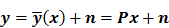
Iteration-based analysis techniques, which comprise the second broad category of statistical analysis techniques, are geared toward reconstruction schemes that are nonconvergent (e.g. some ordered subsets type methods, which offer speedup but do not converge to a stable and unique stationary point) or are terminated early to control noise (e.g. methods seeking to solve an ill-conditioned inverse problem with an unregularized objective function). Unlike fixed-point approaches, for which the stationary point is only dependent on the objective function, for iteration-based approaches, the final reconstructed image is dependent on the objective function, the iterative algorithm used, the image used to initialize the iterative procedure, and the iteration number at which the algorithm is terminated. One of earliest and most significant efforts in this direction was reported by Barrett et al. [12]. This work considers the special case where the EM algorithm is employed to maximize the (unregularized) Poisson likelihood. Denoting the forward model matrix as  and the noise in the data vector as
  , the measured data can be represented as:
The MLEM technique uses an iterative update form that is multiplicative in nature:
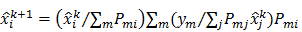
Here  and
and  are the estimates for the
  th voxel intensity at the
  th and
  th iterations respectively and
  is the
  th element of
  . To study the statistics, the multiplicative update is converted to an additive update by taking logarithms:
 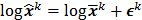 , where
  denotes the mean value of the estimate
  at the
  th iteration and
  represents the corresponding noise vector corrupting the
  th estimate. The first key approximation used in this paper rests on the assumption that the noise in the logarithm of the reconstruction is small. In other words:
The second major approximation is based on the assumption that the projection of the mean value of the current estimate is very close to the projection of the true image. In other words,  . Using these two approximations, the noise in the
  th image estimate can be described by the action of a linear operator
  on the original data noise vector:

where  can be computed from the recursion relation:
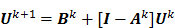
Here  is the identity matrix while the matrices
  and
and  can be computed from the system forward model matrix and the full sequence of noiseless iterates
  . To derive the statistical properties of
  , it is assumed that
  follows a multivariate Gaussian distribution by virtue of the central limit theorem. This assumption is reasonable for PET and SPECT images if the photon count is high enough. Since
  is the result of a linear transformation of
  , it must also follow a multivariate Gaussian distribution. It is therefore possible to derive a closed-form expression for
  , the covariance of
  . The mean and variance of the
  th image estimate can then be computed as:

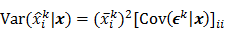
where the notation  denotes the
  th diagonal element of a matrix. These approximate expressions for the mean and variance for MLEM were subsequently compared with Monte Carlo simulation results by Wilson et al. [49]. This study showed that the two approaches have good agreement for high data counts, both for a small number of iterations (corresponding to typical stopping points for MLEM) and for a larger number of iterations.
Similar techniques were applied in [13] to study MAPEM reconstruction, where the EM algorithm is applied to maximize a regularized objective function. Two specific cases were explored in this paper: a MAPEM algorithm for maximizing the Poisson likelihood function augmented by an independent gamma prior and a one-step-late (OSL) version of a MAPEM algorithm incorporating a multivariate Gaussian prior (a more generalized version of the UQP). Monte Carlo validation showed that the approximate expressions for mean and variance agree well with the simulation results if the noise is low (photon counts are high) and bias is low (the regularization parameter is not too large). Similar theoretical derivations were also provided for block-iterative versions of the EM algorithm, including the popular OSEM, in [50].
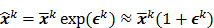
The utility of the iteration-based approaches described above is limited by the fact that they are algorithm specific. Algorithmic modifications would entail derivation of the expressions for the mean and the variance from scratch. Additionally, the mathematical procedure described above only applies to algorithms that perform an explicit multiplicative update. Qi [14] developed a more general framework to analyze noise propagation in images from iteration to iteration. The results are applicable to most gradient-based algorithms and include MLEM, MAPEM, and OSEM as special cases. The framework assumes an additive update equation of the form:

where  is a fixed step size,
  is a positive definite preconditioner matrix, and
  and
and  denote the log likelihood and regularization functions respectively. The noisy data is represented by
  , where
  is the noiseless data vector and
  is the noise vector. The
  th iterate is given by
  , where
  is the noiseless or mean value of this estimate and
  is the noise corrupting it. Using methods similar to [12], a recursive expression can be derived for the noise vector
  , which, in turn, can be used to compute expressions for the mean and covariance. Unlike fixed-point analysis techniques, this “unified” framework does not require the algorithm to be iterated to convergence and therefore is applicable both to algorithms that converge to a fixed point and those that do not. Using this framework Qi [14] demonstrated consistency between fixed-point and iteration-based results. A number of special cases were discussed. These include adaptation of this framework for use with a range of preconditioners (including data-dependent ones). In addition, the results generated by this unified approach were compared with those obtained by iteration-based analysis for MLEM [12], OSL MAPEM [13], and OSEM [10], and any observed discrepancies were explained. Qi [51] further extended this framework to include explicit modeling of line searches and demonstrated improvement in accuracy, especially at early iterations. One limitation of this framework is that it requires the algorithm to have an explicit gradient ascent type update equation. The MAPEM algorithm with the UQP, for example, does not have such an explicit update form. Li [52] developed a unified noise analysis framework that addresses this limitation providing analytical expressions for the mean and covariance matrices for iterative algorithms with implicit update equations.
Applications
Uniform Resolution
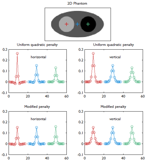
For emission tomographic reconstruction, the UQP, although itself spatially invariant, leads to nonuniform resolution, that (paradoxically) is poorer in high-count regions. This is because, for Poisson statistics, high count regions (which have a high mean activity) also have high variance, which leads to low statistical weights and a relatively large contribution of the penalty. The UQP tends to oversmooth these regions, thereby worsening the local spatial resolution. Uniform resolution is essential for the quantitative interpretation of the reconstructed image and therefore critical for many clinical tasks. To mitigate resolution nonuniformity, a spatially weighted quadratic penalty function was proposed in [27]. The spatially varying weights were data dependent and were computed from approximations for the diagonal elements of the Fisher information matrix for the system. Figure 4 illustrates the improvement in resolution uniformity achieved using this spatially weighted penalty function. The basic approach described in [27] has since been extended for a range of special applications. In [53], a modified version of this method was demonstrated to exhibit count-independent resolution. Perfectly uniform resolution is a lofty goal to strive for due to computational costs. Count-independent resolution seeks to eliminate resolution nonuniformities caused by the spatially varying nature of the activity alone, while nonuniformities due to geometrical and physical factors are allowed to persist. Nevertheless this is a practical and useful technique since the reduction in nonuniformity is significant. A similar technique was reported in [54] for motion-compensated reconstruction. In this case, the resultant spatially varying regularizer was shown to reduce the influence of spatial variation in both activity and degree of deformation on the resolution. In [39], a similar method was described for nonquadratic penalties. Since the LIR is less meaningful for nonquadratic penalties, the focus here is to achieve spatially uniform dependence of the linearized LPR on the applied perturbation.
Horizontal and vertical profiles (concatenated left to right) through the linearized LIRs at the three locations indicated by red, blue, and green markers in the digital phantom (top row). This figure compares the UQP (middle row) and the modified quadratic penalty with spatially modulated weights based on aggregate certainty measures as proposed in [27] (bottom row). Details about the simulated system are provided in the caption for Figure 2. With the UQP, the resolution worsens with increasing activity (from left to right) as revealed by both the horizontal and vertical profiles. The modified penalty mitigates this degradation in resolution. This study is similar to that shown in Figure 4 of [27]. It must be noted that, while Figure 4 of [27] also compares the results of eqs. (6) (circles) and (10) (solid lines), our results are based only on eq. (10).
While the aforementioned techniques reduce the spatial variation in resolution, the achieved resolution is not truly uniform. A more powerful and sophisticated method which accepts any given spatially invariant LIR as an input parameter and generates a customized spatially varying quadratic penalty that leads to the desired LIR was presented in [55] for shift-invariant PET systems, in [56] for shift-variant PET systems, and in [57] for shift-variant SPECT systems. In other words, the objective of the method was to design a matrix  such that the quadratic penalty
  would produce the desired LIR. The way this is done is by starting with a parametric representation for
  in terms of some basis functions and using it to parameterize the LIR. The next step is to perform a least-squares fit of this parameterized LIR to the desired shift-invariant LIR. A computationally efficient Fourier domain approach (based on circulant approximations) was used to determine the basis coefficients for this formulation. Unlike the simpler approach used in [27] which yielded highly anisotropic LIRs, this technique reports uniform and isotropic resolution.
Another important technique that leads to uniform resolution is presented in [31]. As mentioned in the context of fixed-point analysis, this paper reports simple and useful closed-form expressions for the CRC and the variance. The authors took these findings one step further and utilized the expression for the CRC to determine spatial weights for the quadratic penalty that generate a spatially uniform CRC (a measure of resolution). To determine the spatially varying regularization parameter values that lead to uniform resolution, a separate numerical optimization problem had to be solved prior to reconstruction. To accelerate this procedure, the authors proposed a lookup table approach that can significantly alleviate this computational burden, making the technique useful for practical applications.
A simple and effective alternative for generating isotropic resolution based on a continuous space approach was described in [35]. The regularizer design problem is first solved in continuous space and then the solution is discretized for practical implementation. This method for determining spatially varying regularizer weights was intended for a parallel beam emission tomography setup. Several extensions of this method have been reported. These techniques achieve isotropic resolution in 2D fan-beam CT [37], 3D multi-slice axial CT [58], 3D cylindrical PET [38], and motion-compensated PET [45].
Task-Specific Evaluation and Penalty Design
While image quality measures like bias, variance, and resolution are essential for assessing the quantitative accuracy of a reconstruction method, they are not as directly meaningful when the ultimate goal is a specific clinical task. Instead, these image quality measures can be indirectly employed to compute figures of merit which characterize the task of interest. Furthermore, it is possible to use the resultant theoretical analysis to tune reconstruction methods so as to maximize the figure of merit associated with the task of interest.
One common clinical task in PET and SPECT is to quantify the absolute tracer uptake in a given region of interest (ROI). A theoretical analysis of ROI quantitation based on MAP reconstruction is provided in [59]. The derivation of analytical expressions for bias, variance, and ensemble mean squared error (EMSE) for ROI quantitation was based on the Fourier domain approach with circulant approximations described in [31,55,56]. There was generally good agreement between the EMSE values obtained using the analytical expressions and those generated by Monte Carlo simulations. Based on the theoretical approximations, a strategy for selecting the optimum regularization parameter that minimizes the theoretically predicted EMSE was proposed. Wang and Qi [60] further extended these ideas to the context of dynamic PET imaging. The error propagation into kinetic micro- and macroparameters within a given ROI was studied, and approximate analytical expressions for the bias, variance, and EMSE corresponding to these parameters were derived. Once again, this theoretical framework allowed tuning of the regularization parameter so as to minimize the EMSE for the kinetic parameters.
Another common application of PET and SPECT is to ascertain whether a cancerous lesion is present or absent, which is a statistical detection task. The standard tool for quantifying lesion detectability is the receiver operating characteristic (ROC) curve [61,62], which plots the true positive rate against the false positive rate. ROC studies based on human observers, however, can be extremely time-consuming. Computer observers, which employ mathematical models to mimic human performance at a given classification task and offer tremendous savings in time, have therefore become increasingly popular for lesion detection tasks [63,64]. The computational speed enables fast task-based evaluation of different reconstruction schemes. A closed-form expression for the channelized Hotelling observer (CHO) statistic was presented in [65]. The underlying analysis was for MAP reconstruction and utilized the mean and covariance approximations from [32]. Qi and Huesman [66] provided a similar theoretical framework comparing MAP reconstruction with filtered backprojection and deriving closed-form expressions for the SNR for two linear observers, the prewhitening observer and the non-prewhitening (NPW) observer. As humans are not capable of prewhitening the noise in an image [67], the NPW observer is known to better mimic human observer performance than a prewhitening observer. The test statistic SNR for the NPW observer requires an estimate of the noise variance in the image of interest. The derived expressions for the NPW observer SNR in [66] therefore utilized the fixed-point analysis based closed-form variance estimate derived in [31]. A method for designing a shift-invariant quadratic penalty function that maximizes the test statistic SNR for a lesion at a known location using the CHO was presented in [68]. Using both derived analytical expressions and Monte Carlo simulations, it was shown that this method offers improved lesion detectability compared to the UQP and a penalty function that generates isotropic resolution. This method was extended to optimize regularization for lesions at unknown locations in [69]. Theoretical analyses for the performance of linear observer models were performed in [70] for lesions at known locations and in [71] for lesions at unknown locations. These works conclude that, when the lesion location is known, the margin of improvement in detectability offered by optimized regularization over no regularization improves with increasing prewhitening deficiency of the observer.
Optimal Scanner Design
Another critical area where closed-form image quality metrics are beneficial is scanner design optimization. Commonly used figures of merit for scanner design such as spatial resolution, noise equivalent count rate, and noise equivalent sensitivity do not have a direct relationship with the clinical tasks, such as lesion detection, that are often the ultimate goal. A method for optimizing PET scanner design for lesion detection tasks was presented by Qi [72]. The goal of this paper was to determine scanner design parameters that yield the maximum SNR for the NPW observer. The SNR measure from [66] was the basis for the optimization procedure used in [72], which studied the variation in the test statistic SNR with respect to several scanner design parameters for different radial positions for the lesion. Based on the observed SNRs, the author suggested optimal ways to choose the scanner ring diameter, detector transaxial size, and detector radial length.
A method for optimizing the design of a multipinhole SPECT scanner is presented in [73] based on image analysis results for post-smoothed MLEM reconstruction [15,74]. Post-smoothing for MLEM is usually performed using a Gaussian smoothing filter. The image quality measure used as the figure of merit for optimizing the scanner parameters in this paper is the contrast-to-noise ratio (CNR), defined as the ratio of the CRC over the variance. The CRC and variance were computed using approximate expressions derived from fixed-point analysis. For a predefined target resolution, CNR values were computed for practical ranges of values for all the design parameters. Based on this analysis, optimal values were determined for a wide array of parameters, including generic pinhole parameters such as aperture diameter, distance between the apertures and the axis-of-rotation, focal distance, and the acceptance angle as well as multipinhole-specific parameters such as pin radius, focusing distance, and number of pinholes.
Adaptive Systems
Adaptive imaging systems are capable of altering the system hardware configuration in an object-dependent fashion so as to maximize some figure of merit, which is some objective or task-based measure of image quality. The main image acquisition on such systems is preceded by an initial scout image acquisition. Image quality metrics derived from this scout image are used to adjust the configuration for the main scan. Two adaptive small animal pinhole SPECT systems were described in [75]. Two linear observers, the Hotelling observer and the Wiener observer, were considered for task-based image quality measures. The controllable hardware parameters under consideration included the pinhole diameter, the distance of the object center to the pinhole plane, the distance from the pinhole plane to the detector, projection angles, and pinhole pattern in a multiple pinhole configuration.
An adaptive zoom-in PET system was described in [76]. The design of the underlying system, which consisted of a high-resolution detector integrated into a microPET scanner was analyzed in detail in [77]. This design enables high-resolution and high-sensitivity imaging in a small region close to the high-resolution detector. The system model and the data vector for this setup include both the lines of response between the original low-resolution PET detectors and the lines of response between the original PET detectors and the high-resolution detector. Since the positioning of the high-resolution detector can greatly impact localized task performance, the position was set adaptively using a task-based figure of merit. Performance at a lesion detection task was evaluated using the prewhitening observer and the CHO.
Discussion
In this paper, we surveyed quantitative techniques that have been developed for assessing the quality and reliability of iteratively reconstructed images. In spite of the rapid strides made, most of these methods have not reached the clinic. This is because these resources remain largely unexploited in commercially available imaging systems. For commercial systems, the speed of image reconstruction and post-processing steps is of utmost importance. With the limited computer hardware that usually accompanies a typical commercial system today, the computation of a full image covariance matrix or LIRs for each voxel location may be a time-consuming procedure. With the rising popularity of graphical processing units (GPUs) in the image reconstruction and processing communities, computing power will be less of a hurdle in the near future, and thus it would be feasible to assimilate many of the methods discussed herein into onboard data processing routines.
With current computing capabilities, the voxel-wise variance and CRC measures discussed earlier can be computed in a reasonable amount of time. These measures can have a profound impact on quantitation for practical imaging applications. One common scenario where CRC estimates would be helpful is a longitudinal study, where a patient is scanned repeatedly (for example, to monitor disease progression), and tracer uptake at a location (e.g., a lesion) is compared across scans. Based on CRC estimates, image reconstruction or post-smoothing steps can be adjusted to ensure the locations of interest have the same local spatial resolution so that these comparisons are meaningful. The same ideology also applies to studies that involve a population of patients. Voxel-wise variance estimates are critical for quantitative post-processing steps. Pharmacokinetic studies, for example, often rely on accurate estimation of compartment model parameters from dynamic PET scans. The accuracy of these parameters can be greatly improved using accurate voxel-wise variance estimates for the PET images. Even for routine clinical PET scans, voxel-wise variance estimates would enable improved filter design for post-smoothing of the images. Making these quantitative techniques available for more clinical and preclinical imaging applications will greatly facilitate both qualitative interpretation and quantitative analysis of medical images. Whether the application is diagnostics or therapeutics, improved quantitation in medical imaging will ultimately translate to improvement in the quality of life and longevity of patients.
Acknowledgements
This work was funded in part by NIH R21CA149587 and R01EB013293.
Competing Interests
The authors have declared that no competing interest exists.
References
1. Leahy RM, Qi J. Statistical approaches in quantitative positron emission tomography. Stat Comput. 2000;10:147-65
2. Shepp LA, Logan BF. The Fourier reconstruction of a head section. IEEE Trans Nucl Sci. 1974;21:21-43
3. Barrett HH, Swindell W. Radiological imaging: the theory of image formation, detection, and processing. Academic Press. 1996
4. Wilson DW, Tsui BMW. Noise properties of filtered-backprojection and ML-EM reconstructed emission tomographic images. IEEE Trans Nucl Sci. 1993;40:1198-203
5. Kaufman L. Implementing and accelerating the EM algorithm for positron emission tomography. IEEE Trans Med Imaging. 1987;6:37-51
6. Mumcuoglu EÜ, Leahy RM, Cherry SR. Bayesian reconstruction of PET images: methodology and performance analysis. Phys Med Biol. 1996;41:1777-808
7. Fessler JA, Ficaro EP. Fully 3D PET image reconstruction using a Fourier preconditioned conjugate-gradient algorithm. IEEE Nucl Sci Symp Conf Rec. 1996:1599-602
8. Shepp LA, Vardi Y. Maximum likelihood reconstruction for emission tomography. IEEE Trans Med Imaging. 1982;1:113-22
9. Lange K, Carson R. EM reconstruction algorithms for emission and transmission tomography. J Comput Assist Tomogr. 1984;8:306-16
10. Hudson HM, Larkin RS. Accelerated image reconstruction using ordered subsets of projection data. IEEE Trans Med Imaging. 1994;13:601-9
11. Browne J, De Pierro AB. A row-action alternative to the EM algorithm for maximizing likelihood in emission tomography. IEEE Trans Med Imaging. 1996;15:687-99
12. Barrett HH, Wilson DW, Tsui BMW. Noise properties of the EM algorithm: I Theory. Phys Med Biol. 1994;39:833-846
13. Wang W, Gindi G. Noise analysis of MAP-EM algorithms for emission tomography. Phys Med Biol. 1997;42:2215-2232
14. Qi J. A unified noise analysis for iterative image estimation. Phys Med Biol. 2003;48:3505-19
15. Nuyts J. On estimating the variance of smoothed MLEM images. IEEE Trans Nucl Sci. 2002;49:714-21
16. Dempster AP, Laird NM, Rubin DB. Maximum likelihood from incomplete data via the EM algorithm. J R Stat Soc Series B Stat Methodol. 1977;39:1-38
17. Fessler JA, Hero III AO. Penalized maximum-likelihood image reconstruction using space-alternating generalized EM algorithms. IEEE Trans Image Process. 1995;4:1417-29
18. Byrne CL. Accelerating the EMML algorithm and related iterative algorithms by rescaled block-iterative methods. IEEE Trans Image Process. 1998;7:100-9
19. De Pierro AR, Yamagishi MEB. Fast EM-like methods for maximum "a posteriori" estimates in emission tomography. IEEE Trans Med Imaging. 2001;20:280-8
20. Llacer J, Veklerov E. Feasible images and practical stopping rules for iterative algorithms in emission tomography. IEEE Trans Med Imaging. 1989;8:186-93
21. Llacer J, Veklerov E, Coakley KJ, Hoffman EJ, Nunez J. Statistical analysis of maximum likelihood estimator images of human brain FDG PET studies. IEEE Trans Med Imaging. 1993;12:215-31
22. Fessler JA. Penalized weighted least-squares image reconstruction for positron emission tomography. IEEE Trans Med Imaging. 1994;13:290-300
23. Bouman CA, Sauer K. A unified approach to statistical tomography using coordinate descent optimization. IEEE Trans Image Process. 1996;5:480-92
24. Hero III AO, Fessler JA, Usman M. Exploring estimator bias-variance tradeoffs using the uniform CR bound. IEEE Trans Signal Process. 1996;44:2026-41
25. Meng LJ, Clinthorne NH. A modified uniform Cramer-Rao bound for multiple pinhole aperture design. IEEE Trans Med Imaging. 2004;23:896-902
26. Stamos JA, Rogers WL, Clinthorne NH, Koral KF. Object-dependent performance comparison of two iterative reconstruction algorithms. IEEE Trans Nucl Sci. 1988;35:611-4
27. Fessler JA, Rogers WL. Spatial resolution properties of penalized-likelihood image reconstruction: space- invariant tomographs. IEEE Trans Image Process. 1996;5:1346-58
28. Fessler JA. Mean and variance of implicitly defined biased estimators (such as penalized maximum likelihood): Applications to tomography. IEEE Trans Image Process. 1996;5:493-506
29. De Pierro AR. A modified expectation maximization algorithm for penalized likelihood estimation in emission tomography. IEEE Trans Med Imaging. 1995;14:132-7
30. Lalush DS, Tsui BMW. A fast and stable maximum a posteriori conjugate gradient reconstruction algorithm. Med Phys. 1995;22:1273-84
31. Qi J, Leahy RM. Resolution and noise properties of MAP reconstruction for fully 3-D PET. IEEE Trans Med Imaging. 2000;19:493-506
32. Qi J, Leahy RM. A theoretical study of the contrast recovery and variance of MAP reconstructions from PET data. IEEE Trans Med Imaging. 1999;18:293-305
33. Fessler JA, Booth SD. Conjugate-gradient preconditioning methods for shift-variant PET image reconstruction. IEEE Trans Image Process. 1999;8:688-99
34. Li Q, Asma E, Qi J, Leahy RM. Accurate estimation of the Fisher information matrix for the PET image reconstruction problem. IEEE Trans Med Imaging. 2004;23:1057-64
35. Fessler JA. Analytical approach to regularization design for isotropic spatial resolution. IEEE Nucl Sci Symp Conf Rec. 2003:2022-6
36. Zhang-O'Connor Y, Fessler JA. Fast predictions of variance images for fan-beam transmission tomography with quadratic regularization. IEEE Trans Med Imaging. 2007;26:335-46
37. Shi HR, Fessler JA. Quadratic regularization design for 2-D CT. IEEE Trans Med Imaging. 2009;28:645-56
38. Shi HR, Fessler JA. Quadratic regularization design for 3D cylindrical PET. IEEE Nucl Sci Symp Conf Rec. 2005:2301-5
39. Ahn S, Leahy RM. Analysis of resolution and noise properties of nonquadratically regularized image reconstruction methods for PET. IEEE Trans Med Imaging. 2008;27:413-24
40. Asma E, Leahy RM. Mean and covariance properties of dynamic PET reconstructions from list-mode data. IEEE Trans Med Imaging. 2006;25:42-54
41. Carson RE. Tracer Kinetic Modeling in PET. Bailey DL, Townsend DW, Valk PE, Maisey MN. Positron Emission Tomography: Basic Sciences. Springer. 2005:127-59
42. Nehmeh SA, Erdi YE, Pan T, Pevsner A, Rosenzweig KE, Yorke E. et al. Four-dimensional (4D) PET/CT imaging of the thorax. Med Phys. 2004;31:3179-86
43. Klein GJ, Reutter BW, Ho MH, Reed JH, Huesman RH. Real-time system for respiratory-cardiac gating in positron tomography. IEEE Trans Nucl Sci. 1998;45:2139-43
44. Dutta J, El Fakhri G, Huang C, Petibon Y, Reese TG, Li Q. Respiratory motion compensation in simultaneous PET/MR using a maximum a posteriori approach. Proc, IEEE Int Symp Biomed Imaging. 2013:788-91
45. Chun SY, Fessler JA. Spatial resolution properties of motion-compensated tomographic image reconstruction methods. IEEE Trans Med Imaging. 2012;31:1413-25
46. Chun SY, Fessler JA. Noise properties of motion-compensated tomographic image reconstruction methods. IEEE Trans Med Imaging. 2013;32:141-52
47. Haldar JP, Liang Z-P. On MR experiment design with quadratic regularization. Proc, IEEE Int Symp Biomed Imaging. 2011:1676-9
48. Khalsa KA, Fessler JA. Resolution properties in regularized dynamic MRI reconstruction. Proc, IEEE Int Symp Biomed Imaging. 2007:456-9
49. Wilson DW, Tsui BMW, Barrett HH. Noise properties of the EM algorithm: II Monte Carlo simulations. Phys Med Biol. 1994;39:847-71
50. Soares EJ, Byrne CL, Glick SJ. Noise characterization of block-iterative reconstruction algorithms: I Theory. IEEE Trans Med Imaging. 2000;19:261-70
51. Qi J. Noise propagation in iterative reconstruction algorithms with line searches. IEEE Trans Nucl Sci. 2005;52:57-62
52. Li Y. Noise propagation for iterative penalized-likelihood image reconstruction based on Fisher information. Phys Med Biol. 2011;56:1083-103
53. Li Q, Bai B, Cho S, Smith A, Leahy RM. Count Independent Resolution and Its Calibration. 10th International Meeting on Fully Three-Dimensional Image Reconstruction in Radiology and Nuclear Medicine, Proceedings. 2009:223-4
54. Dutta J, El Fakhri G, Lin Y, Huang C, Petibon Y, Reese TG. et al. Spatially varying regularization for motion compensated PET reconstruction. IEEE Nucl Sci Symp Conf Rec. 2012:2156-60
55. Stayman JW, Fessler JA. Regularization for uniform spatial resolution properties in penalized-likelihood image reconstruction. IEEE Trans Med Imaging. 2000;19:601-15
56. Stayman JW, Fessler JA. Compensation for nonuniform resolution using penalized-likelihood reconstruction in space-variant imaging systems. IEEE Trans Med Imaging. 2004;23:269-84
57. Stayman JW, Fessler JA. Efficient calculation of resolution and covariance for penalized-likelihood reconstruction in fully 3-D SPECT. IEEE Trans Med Imaging. 2004;23:1543-56
58. Shi HR, Fessler JA. Quadratic regularization design for iterative reconstruction in 3D multi-slice axial CT. IEEE Nucl Sci Symp Conf Rec. 2006:2834-6
59. Qi J, Huesman RH. Theoretical study of penalized-likelihood image reconstruction for region of interest quantification. IEEE Trans Med Imaging. 2006;25:640-8
60. Wang G, Qi J. Analysis of penalized likelihood image reconstruction for dynamic PET quantification. IEEE Trans Med Imaging. 2009;28:608-20
61. Gilland DR, Tsui BMW, Metz CE, Jaszczak RJ, Perry JR. An evaluation of maximum likelihood-expectation maximization reconstruction for SPECT by ROC analysis. J Nucl Med. 1992;33:451-7
62. Llacer J. Results of a clinical receiver operating characteristic study comparing filtered backprojection and maximum likelihood estimator images in FDG PET studies. J Nucl Med. 1993;34:1198-203
63. Barrett HH, Yao J, Rolland JP, Myers KJ. Model observers for assessment of image quality. Proc Natl Acad Sci. 1993;90:9758-65
64. Barrett HH, Myers KJ, Rathee S. Foundations of image science. Wiley New York. 2004
65. Bonetto P, Qi J, Leahy RM. Covariance approximation for fast and accurate computation of channelized Hotelling observer statistics. IEEE Trans Nucl Sci. 2000;47:1567-72
66. Qi J, Huesman RH. Theoretical study of lesion detectability of MAP reconstruction using computer observers. IEEE Trans Med Imaging. 2001;20:815-22
67. Myers KJ, Barrett HH, Borgstrom MC, Patton DD, Seeley GW. Effect of noise correlation on detectability of disk signals in medical imaging. J Opt Soc Am A Opt Image Sci Vis. 1985;2:1752-9
68. Qi J, Huesman RH. Penalized maximum-likelihood image reconstruction for lesion detection. Phys Med Biol. 2006;51:4017-29
69. Yang L, Zhou J, Qi J. Regularization design for breast lesion detection in penalized maximum likelihood image reconstruction. Proc, IEEE Int Symp Biomed Imaging. 2012:626-629
70. Yendiki A, Fessler JA. Analysis of observer performance in known-location tasks for tomographic image reconstruction. IEEE Trans Med Imaging. 2006;25:28-41
71. Yendiki A, Fessler JA. Analysis of observer performance in unknown-location tasks for tomographic image reconstruction. J Opt Soc Am A Opt Image Sci Vis. 2007;24:B99-B109
72. Qi J. Optimization of PET system design for lesion detection. IEEE Trans Nucl Sci. 2001;48:1470-6
73. Vunckx K, Bequé D, Defrise M, Nuyts J. Single and multipinhole collimator design evaluation method for small animal SPECT. IEEE Trans Med Imaging. 2008;27:36-46
74. Nuyts J, Fessler JA. A penalized-likelihood image reconstruction method for emission tomography, compared to postsmoothed maximum-likelihood with matched spatial resolution. IEEE Trans Med Imaging. 2003;22:1042-52
75. Barrett HH, Furenlid LR, Freed M, Hesterman JY, Kupinski MA, Clarkson E, Whitaker MK. Adaptive SPECT. IEEE Trans Med Imaging. 2008;27:775-88
76. Zhou J, Qi J. Adaptive imaging for lesion detection using a zoom-in PET system. IEEE Trans Med Imaging. 2011;30:119-30
77. Zhou J, Qi J. Theoretical analysis and simulation study of a high-resolution zoom-in PET system. Phys Med Biol. 2009;54:5193-208
Author contact
![]() Corresponding author: Quanzheng Li, 55 Fruit St, White 427, Boston MA 02114, USA. Tel: 1(617)643-9481, Fax: 1(617)726-6165, Email: Li.Quanzhengharvard.edu.
Corresponding author: Quanzheng Li, 55 Fruit St, White 427, Boston MA 02114, USA. Tel: 1(617)643-9481, Fax: 1(617)726-6165, Email: Li.Quanzhengharvard.edu.