Impact Factor
 Global reach, higher impact
Theranostics 2018; 8(1):277-291. doi:10.7150/thno.22065 This issue Cite
Research Paper
Tiresias: Context-sensitive Approach to Decipher the Presence and Strength of MicroRNA Regulatory Interactions
Jinkyu Koo1, Jinyi Zhang2, Somali Chaterji3 ![]()
1. Electrical and Computer Engineering, Purdue University, West Lafayette, IN, USA;
2. Computer Science, Columbia University, New York, NY, USA;
3. Computer Science, Purdue University, West Lafayette, IN, USA.
Received 2017-7-24; Accepted 2017-10-9; Published 2018-1-1
Abstract

MicroRNAs (miRNAs) are short non-coding RNAs that regulate expression of target messenger RNAs (mRNAs) post-transcriptionally. Understanding the precise regulatory role of miRNAs is of great interest since miRNAs have been shown to play an important role in development, diseases, and other biological processes. Early work on miRNA target prediction has focused on static sequence-driven miRNA-mRNA complementarity. However, recent research also utilizes expression-level data to study context-dependent regulation effects in a more dynamic, physiologically-relevant setting.
Methods: We propose a novel artificial neural network (ANN) based method, named Tiresias, to predict such targets in a context-dependent manner by combining sequence and expression data. In order to predict the interacting pairs among miRNAs and mRNAs and their regulatory weights, we develop a two-stage ANN and present how to train it appropriately. Tiresias is designed to study various regulation models, ranging from a simple linear model to a complex non-linear model. Tiresias has a single hyper-parameter to control the sparsity of miRNA-mRNA interactions, which we optimize using Bayesian optimization.
Results: Tiresias performs better than existing computational methods such as GenMiR++, Elastic Net, and PIMiM, achieving an F1 score of >0.8 for a certain level of regulation strength. For the TCGA breast invasive carcinoma dataset, Tiresias results in the rate of up to 82% in detecting the experimentally-validated interactions between miRNAs and mRNAs, even if we assume that true regulations may result in a low level of regulation strength.
Conclusion: Tiresias is a two-stage ANN, computational method that deciphers context-dependent microRNA regulatory interactions. Experiment results demonstrate that Tiresias outperforms existing solutions and can achieve a high F1 score. Source code of Tiresias is available at
Keywords: MicroRNA, messenger RNA, machine learning, artificial neural networks, Bayesian optimization, breast cancer, condition-specific regulation.
Introduction
MicroRNAs (miRNAs) are non-coding RNAs of ~22-nucleotide length that can regulate gene expression by binding to complementary sequences on target messenger RNAs (mRNAs). So far, only part of the hundreds of known human miRNAs have been experimentally linked to their target mRNAs. Accurately determining the entire miRNA targetome is a major bottleneck in miRNA functional characterization, which is important in unraveling disease mechanisms and determining the efficacy of drugs.
The first generation of computational methods developed to predict miRNA targets are primarily based on nucleotide-sequence information [1-4]. Such computational methods mainly utilize the sequence complementarity between the seed region of the miRNAs, mostly situated at nucleotides 2-7 from the miRNA 5'-end, and the 3'-UTR of the mRNAs. However, in the sequence-based genre of miRNA targeting algorithms, it was later realized that sequence complementarity was neither necessary nor sufficient for the miRNA-mRNA interactions to occur, which was further validated by the presence of a vast swath, specifically >90%, of these so-called non-canonical interactions [5]. These interactions were deciphered from the datasets obtained from high-throughput sequencing (CLIP-seq) experiments, such as, PAR-CLIP (Photoactivatable Ribonucleoside-Enhanced Crosslinking and Immunoprecipitation) and HITS-CLIP (High-throughput sequencing of RNA isolated by crosslinking immunoprecipitation). In fact, our recent work where we used both sequence and thermodynamic features at two levels of granularity—seed level (finer granularity) and site level (coarser granularity around the miRNA-mRNA interaction site)—resulted in superior prediction of these non-canonical interaction sites [6]. Our prediction performance improved further when using a non-linear kernel for our classifier, reducing the bias in our simpler linear model, with an improvement of >150% in the true positive rate for non-canonical sites, over the best competitive protocol [7], and validated using cancer-specific data. These methods are simple and useful to build a putative interaction database, but they are far from perfect, leading to many false positives and some false negatives.
Unlike sequence data, expression data is context-specific and, in one sense, dynamic, providing useful clues on regulation effects that may vary depending on conditions, such as time, pathophysiology, and cell-type (spatial) context. Thus, context-dependent regulation can be found by analyzing expression data. Correlation analyses including Pearson correlation coefficient (PCC) were initially attempted with the expression data [8], measuring the strength of interactions between miRNAs and mRNAs. However, correlation-based detection leads to a high error rate, since correlation coefficients of interacting pairs can be small, falling in the measurement error range, unless the regulation relationship is strong. In addition, these methods cannot adequately model the demonstrated joint effects of several miRNAs on a shared mRNA target. To account for the joint effects of multiple miRNAs on an mRNA, multiple linear regression models with regularization have been proposed. Lasso regression [9] and Elastic Net regression [10] fall into this category. However, they can only provide a sparse solution, i.e., a relatively small set of strong interactions.
Recently, utilizing both sequence and expression data is getting much attention. Representative work is a variational inference model considered in GenMiR++ [11, 12]. The aim of this model is to infer the probabilities of putative targets of being real by approximating the posterior with variational inference techniques. A drawback of this approach is that the expectation maximization (EM) algorithm involved in variational inference is computationally expensive. Further, the search space for the parameters is restricted to be in the realm of down-regulation only. A probabilistic regression model in [13], called PIMiM, introduced a group-based regulatory model, based on both sequence and expression data. This method can form groups of miRNAs and mRNAs that may function together, but is hard to optimize in practice due to its large number of hyper-parameters, e.g., the numbers of groups, miRNAs per group, and mRNAs per group. On the other hand, recent research results are reporting that up-regulations also exist [14] and non-linear regulation relationship fits better to real data in some cases [15,16]. However, existing computational methods cannot be easily extended to study non-linear regulation models because the problem formulation will look significantly different. Thus, we need a new method that can reflect the above scenarios.
To address the above challenges, we propose Tiresias in this paper.1 Tiresias is a new explanatory computational method based on artificial neural networks (ANNs) that analyzes a given dataset, and finds miRNA targets under context-specific conditions by incorporating expression-level data into sequence-based prediction results. Tiresias decouples the problem in a manner that makes the learning easier—the first stage estimates miRNA targets and the second stage estimates the regulation weight based on the previous stage outputs. Tiresias considers up-regulation as well as down-regulation, simultaneously. By virtue of the ANN-based approach, Tiresias can easily remove the assumption of linear regulation, extending it to a complex non-linear regulation model. Thus, Tiresias can support multiple variations in modeling, from each of which we can get insights understanding regulation relationship hiding underneath complex biological processes. Tiresias characterizes the density of miRNA-mRNA interactions using one single hyper-parameter unlike the most relevant prior work [13], which uses a large number of hyper-parameters, e.g., to individually control for how many miRNAs belong to a group. This design makes Tiresias a good fit for Bayesian optimization by which we optimize the hyper-parameter in a way that a regression error is minimized.
We compare Tiresias to a variational inference model, GenMiR++ [12], an Elastic Net regression method [10], and a probabilistic regression approach, called PIMiM [13], all of which, like Tiresias, are well suited to high-dimensional biological data. Our experiments using synthetic data show that Tiresias significantly improves upon these prior methods, and can achieve a F1 score > 0.8, that is, a high true positive rate and a low false positive rate, in predicting regulatory interactions, which are stronger than a certain threshold. Using real breast cancer datasets from the Cancer Genome Atlas (TCGA) [17], Tiresias shows a detection rate of up to 82% in recovering the experimentally-validated interactions between miRNAs and mRNAs, even if we assume that regulations may result in small values of PCC for the interacting miRNA-mRNA pairs.
Methods
Regulation model
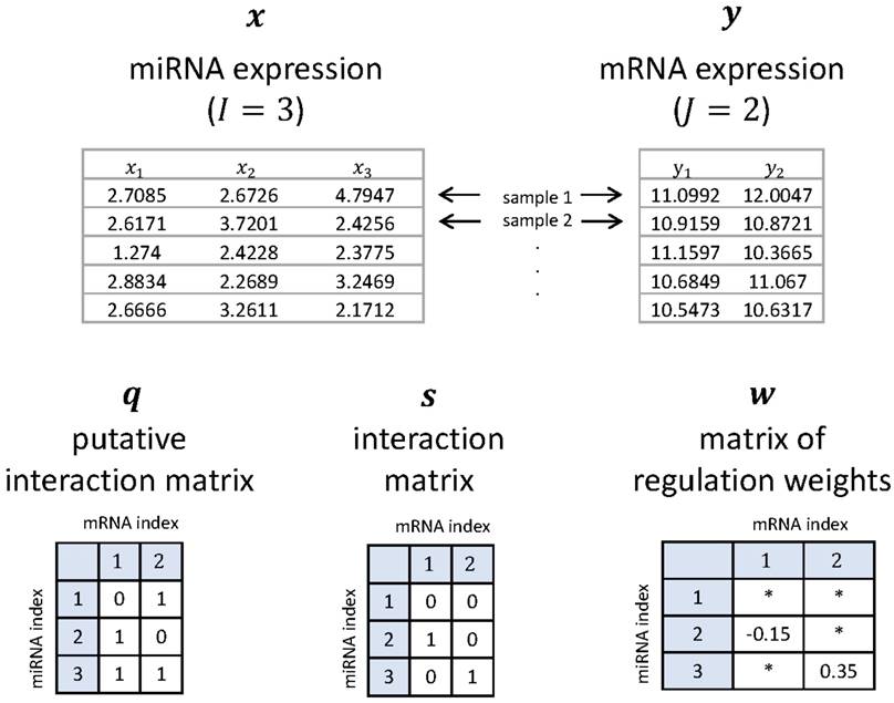
We consider a set of expression-level data that consists of I miRNAs and J mRNAs. We denote a sample of an miRNA expression vector by x = (xi) ∈ RI×1 where xi is the expression of the i-th miRNA of the sample and R denotes the set of real numbers, and a corresponding sample of an mRNA expression vector by y = (yj) ∈ RJ×1 where yj is the expression of the j-th mRNA. We assume that yj for any j is normally distributed, and the relationship between yj and x can be described as
, (1)
where μj > 0 is the background mean of yj, i.e., the mean of yj when it is not regulated by any miRNA, and  is the variance of yj. The normality assumption for expression values just comes from the law of large numbers [18]. Later, we will see that this assumption does not need to hold strictly. The rj(x,s) is a regulation function that determines the amount of regulation on yj by x, given an interaction matrix s defined as s = (sij) ∈ {0,1}I×J. Here, sij, the entry in the i-th row and j-th column of the I × J matrix s is set as sij = 1 if yj is regulated by xi, and as sij = 0 otherwise.
In this paper, we mainly consider the following regulation model2:
, (2)
where wij ∈ R is a regulation weight that rules the relative strength of regulation on yj due to xi. Note that a positive value of wij means up-regulation, and a negative wij is down-regulation. On the other hand, qij ∈ {0,1} is a putative-interaction indicator, built by a nucleotide-sequence-level predictor like TargetScan [2], with qij = 1 meaning possible interaction. We call q = (qij) ∈ {0,1}I×J the putative interaction matrix. The q is made available based on miRNA-target site complementarity allowing some mismatches, and qij = 1 can be considered to be a necessary condition for sij = 1. Typically, q contains much more 1's as its elements than s, i.e., false positives. What we want to do in this paper can be understood as getting rid of the false positives from sequence-based prediction results and filtering out only true positives with their regulation strength and direction. Figure 1 shows a simple example to help understand our notations.
A simple example for the miRNA vector x, the mRNA vector y, the putative interaction matrix q, the interaction matrix s, and the matrix w of regulation weights when I = 3 and J = 2. Here, '*' denotes a 'don't care' value.
Thus, our goal is to find wij and sij for all i,j that maximize the posterior probability density function (pdf),
(3)
subject to μj > 0 for all j where w = (wij) ∈ RI×J and μ = (μj) ∈ RJ×1, and eventually to compute what we call the regulatory network edge matrix, e = (eij) ∈ RI×J where eij is an estimate of wijsij. That is, we want to represent the regulatory network as an edge eij between xi and yj that is an estimate of wijsij.
Regulation weight estimation network
Consider a function vector f(x,s) ∈ RJ×1 whose j-th element fj(x,s) is defined as
. (4)
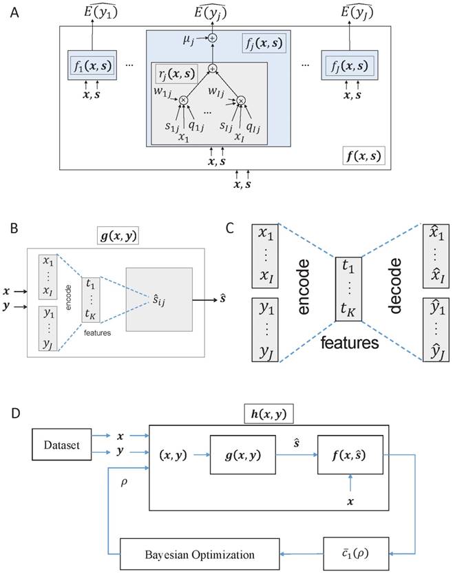
The f(x,s) can be regarded as an ANN shown in Figure 2A that takes x and s as its input and produces fj(x,s) as an estimate  for the mean of yj for all j.3
(A) Regulation weight estimation network f(x,s), where x is a sample of the miRNA expression vector, and s is the interaction matrix. Training this network without knowing a reasonably good estimate of s will not result in any meaningful regulation weights at all. (B) The miRNA target estimation network g(x,y) that takes x and y as inputs, and is intended to result in  as the estimate of the ground truth interaction matrix s given x and y. Training this network alone just produces a random matrix whose entry is close to 0 or 1, which is far from an appropriate estimate of s given x and y. (C) An autoencoder where the features are extracted by training the network in such a way that
  and
and  are, respectively, produced as close to xi and yj as possible. (D) Overall architecture of Tiresias. For a given value of ρ, f(x,s) and g(x,y) are trained together for the whole data sample pairs of x and y. The Bayesian optimization tunes the value of ρ based on
  .
.
Assuming that the interaction matrix s is given, the regulation weights wij's (and the background means μj 's) that maximize Equation (3) can be found by training the ANN f(x,s) in a way that minimizes the cost function c(x,y) defined as:
(5)
where λ1 > 0 is a penalty weight. Note in Equation (5) that the first term comes from -lnp(y|x;w,s,μ), and the second term is a penalty that becomes a positive value if μj < 0 for any j, and remains zero otherwise. From the first term in Equation (5), we can also think of fj(x,s) as a regression function that fits to yj, minimizing the mean squared error (MSE) between yj and fj(x,s), which can be done without knowing the distribution of yj. Thus, even though the normality assumption in (1) does not hold, Tiresias works as an MSE-based regression method, which we will see in experiment results.
Since we can find wij's from f(x,s) in that way, we call f(x,s) the regulation weight estimation network. Not to mention, the accuracy of the estimated value of wij is highly dependent on the correctness of s that we assumed to be given earlier. However, the ground truth of s is typically not available or is imperfect in practice. Thus, we design another ANN to estimate s given x and y, which is described in the following section.
miRNA Target Estimation Network
We denote an estimator of s given x and y by ŝ = g(x,y). Then, we define ŝ as ŝ = (ŝij) ∈ [0,1] I×J, where
(6)
with a(z) = 1/(1+exp(-z)) meaning a sigmoid activation function shown in Figure S1A of Supplementary material, and uijk ∈ R for any k meaning a coefficient from tk to ŝij. The sat(z) is what we call a saturation function and defined as sat(z) = 0.5tanh(10(z-0.5))+0.5 (shown in Figure S1B of Supplementary material), which is intended to make the value of ŝij more likely to be 0 or 1. The tk for any k denotes a feature extracted from both x and y using an autoencoder [19, 20], and is expressed as
(7)
in which bkp ∈ R and b'kp ∈ R for any k,p.4 The K is the number of the features extracted from x and y, the value of which is chosen to be much smaller than I + J, e.g., we can set K = 1 or 2 (see Figure 5E). Thus, g(x,y) is an ANN depicted in Figure 2B that has x and y as input, and results in ŝ whose (i,j) entry ŝij is the estimate of sij given x and y, i.e., P(sij = 1|x,y). Since ŝij is the output of the saturation function, we have 0 ≤ ŝij ≤ 1. We call g(x,y) the miRNA target estimation network.
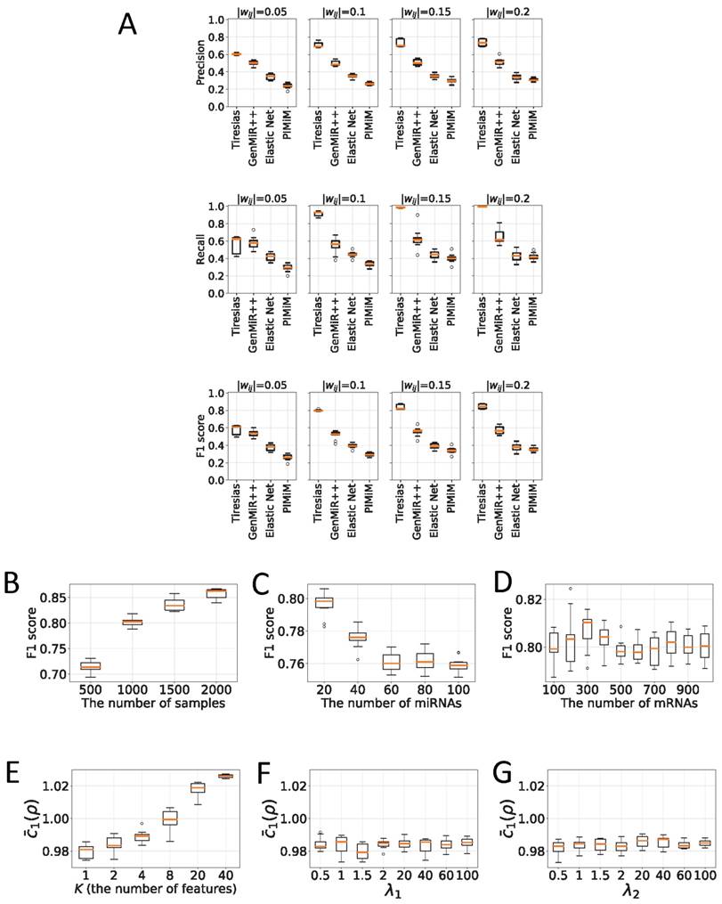
(A) Box plots for precision, recall, and F1 score showing performance of Tiresias versus GenMiR++, Elastic Net, and PIMiM. Tiresias significantly outperforms others in all measures except at |wij| = 0.05. (B)-(D) Tiresias's F1 score with increase in the number of samples, miRNAs, and mRNAs (|wij| = 0.10 for ground-truth pairs). Performance improves with the increase in samples. Increase in the number of miRNAs or mRNAs means a higher level of noise, which results in performance degradation. We can also see that increase in J makes little impact on performance, compared to increase in I. (E)-(G) Effects of internal parameters. Tiresias is trained better with a smaller value of K. Choices for the values of λ1 and λ2 are not critical.
All the coefficients in Equation (7) are pre-trained by an autoencoder shown in Figure 2C, in such a way that the autoencoder output  gets as close to (x,y) as possible. Thus, when we train g(x,y), we mainly need to find a single layer of coefficients uijk in Equation (6), although g(x,y) is effectively an ANN of two activation layers. The rationale behind this design is that we introduce a large enough number of activation layers to make it possible for g(x,y) to exhibit non-linear behavior, if necessary, and we make the training of g(x,y) easier by reducing the number of unknown coefficients.
We train the ANN g(x,y) by mainly minimizing the Kullback-Leibler divergence from  to ρ,
to ρ,
(8)
where
(9)
and ρ < 1 is a sparsity parameter that controls how many of ŝij's activate (i.e., come close to 1) on an average. The  has the property that
  if
if  , and otherwise it grows monotonically as
  diverges from ρ. Thus, by minimizing the
  in Equation (8), we can make only 100ρ percent of elements of ŝ become close to 1, which are mostly located at where putative interaction is expected, and the remaining get close to 0.
Note that, so far, ŝij does not have much relationship with P(sij = 1|x,y), although we call ŝ the estimate of s given x and y. Minimizing Equation (8) alone will result in ŝ that is more or less a random matrix whose elements are close to 1 or 0, except that most of ŝij's that are close to 1 are the entries where qij = 1. In order to make ŝij a meaningful estimate of P(sij = 1|x,y), we need a way to relate ŝ and p(y|x;w,s,μ). The next section explains such a method.
Training the estimation networks
We have introduced two ANNs, f(x,s) and g(x,y). However, training f(x,s) cannot be done without the estimate of s beforehand, and training g(x,y) alone will not produce a meaningful estimate of s given x and y. In other words, neither of the two ANNs can be trained independently. So as to train f(x,s) and g(x,y) in a proper way, we consider h(x,y) shown in Figure 2D, a concatenated network of g(x,y) and f(x,s). In h(x,y), the output ŝ of g(x,y) is fed into f(x,s) as s = ŝ. We train h(x,y) as a single ANN by minimizing the cost function c'(x,y) defined as:
(10)
which is simply a weighted sum of Equation (5) and Equation (8) with a weight λ2 > 0.
Note that although the term  in Equation (10) is computed at the end of f(x,s), the gradient of this portion of the cost can be transferred to g(x,y) by backpropagation [21], since the output of g(x,y) is connected with f(x,s) by multiplication. Thus, training h(x,y) leads to g(x,y) trained in such a way that the number of activated elements in ŝ is controlled by ρ, just as we intended. By the other terms in Equation (10), g(x,y) is also trained toward maximizing the posterior pdf p(y|x;w,s,μ). That way, g(x,y) gets related with p(y|x;w,s,μ), and in turn, produces a legitimate estimate of s that maximizes Equation (3).
On the other hand, the regulation weights of f(x,s) can also be found by training h(x,y) at the same time, because in this setup of h(x,y), the f(x,s) is getting ŝ as an estimate of s from g(x,y). As ŝ approaches a meaningful one, f(x,s) also results in meaningful regulation weights.
For training h(x,y), we can select from a suite of optimization techniques. For example, if we use the stochastic gradient descent, the value of wij should be updated until convergence as:
(11)
for a given sample pair of x and y, where α > 0 is called a learning rate and should be small enough for convergence. The other remaining unknowns of h(x,y), i.e., uijk and μj are also updated in a similar manner as Equation (11).
Bayesian optimization
In h(x,y), ρ is a hyper-parameter such that ρ is a variable that is not learned by training h(x,y), but affects how h(x,y) works.5 A proper choice of ρ, i.e., as close as possible to the ground truth value, is the key to achieving good accuracy of our estimation networks.
For this reason, we find the optimal value of ρ, denoted by ρ*, using the Bayesian optimization framework, as illustrated at the bottom of Figure 2D. We define ρ* as the one that minimizes the following on average:
(12)
which is the first term of c'(x,y) in Equation (10). Roughly speaking, ρ* can thus be said to be the value of ρ that maximizes Equation (3) without considering any penalty terms in Equation (10), which are usually negligible when training h(x,y) is done for a given value of ρ. In practice, c1(x,y) keeps fluctuating near a converging point while training. Thus, we instead consider  , the average of the last few hundreds of sample values for c1(x,y) while training h(x,y) for a certain value of ρ. The Bayesian optimization helps us efficiently choose the next value of ρ to examine, based on the resulting history of
  , which corresponds to the values of ρ that we have tried so far, and ultimately find the optimal value ρ*.
In effect, we first try a few random guesses for ρ, train h(x,y) for each guess using the same dataset, and observe the resulting values for  . Based on this history about the values of ρ and corresponding
  , a Bayesian optimization solver decides on the next value of ρ to evaluate. Then, we train h(x,y) again using this value of ρ and observe the new value of
  . Such a process keeps repeating until our termination criterion is met.
The decision on the new value of ρ to try is made by compromising the trade-off between exploration and exploitation. Exploration means we try new values where  is very uncertain, but could lead to improvement. Exploitation means we choose the new value in the vicinity of prior desirable values of ρ, i.e., where we have some certainty that
  is expected to be low. By this approach, we can minimize the number of evaluations of
  , each of which corresponds to training h(x,y) for the whole dataset of sample pairs of x and y, which is an expensive operation. The details of the Bayesian optimization process is out of scope for this paper and interested readers may refer to [22] for details.
Data scaling
Since we are analyzing interaction relationships among multiple miRNAs and mRNAs simultaneously, data scaling that standardizes the range of each miRNA or mRNA is important. Without such scaling, the cost function during training is governed by few specific miRNAs or mRNAs that have a broad range or a large magnitude of values, and eventually, we end up with poorly trained ANNs. Thus, all the datasets considered in this paper are scaled appropriately. Details for this are presented in Section S1 of Supplementary material.
Summary of Tiresias
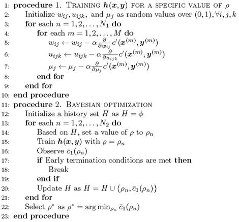
The whole procedure to train Tiresias is summarized in Figure 3, assuming that we use the stochastic gradient descent as an optimization method. The procedure 1 corresponds to training h(x,y) for a given value of ρ, where M is the number of sample pairs of x and y, and the superscript (m) over x and y means the m-th sample of them. For each data sample pair, the unknowns of h(x,y) are updated toward convergence by lines 5 to 7, and these updates can be repeated N1 times (line 3) as typically required in the stochastic gradient descent when M is not large enough. The procedure 2 explains how to find the optimal value of ρ using Bayesian optimization. We train h(x,y) for a selected value of ρ (line 15), observe  (line 16), and update a history set H about ρ and
  (line 20). Based on the history set H, the next value of ρ to try is decided (line14) using a tradeoff between exploration and exploitation. This process is repeated N2 times (line 13) before early termination conditions are met (line 18). The early termination conditions could be whether
  is low enough, or whether
  gets larger than its historical minimum in a row. The optimal value ρ* is determined to be the value of ρ that results in the minimum for
  (line 22).
Pseudo code that shows how to train Tiresias.
After we complete training Tiresias through procedures in Figure 3, we use the converged values of unknowns of h(x,y) that result from ρ* in order to finalize the regulatory network edge matrix e. We determine e as:
, (13)
where  implies the element-wise product (also known as the Schur product) between two matrices a and b. In other words, the edge eij of the regulatory network is the estimate of wijsij that we compute as:
(14)
assuming that P(x(m),y(m)) = 1/M.
Note that Tiresias is not predicting an interaction for a new data sample after training, but it figures out the interaction from the dataset by which it is trained. Namely, Tiresias is an explanatory model that analyzes the given dataset and finds out the potential regulatory interactions. Thus, the overfitting to the training data that is an issue of a predictive model is not relevant here [23].
Extension to non-linear regulation models
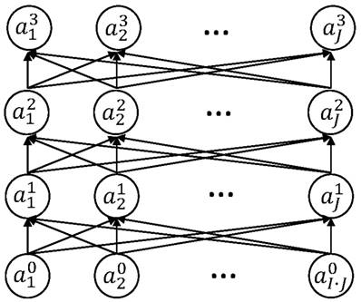
In Tiresias, the regulation model rj(x,s) is a sub-network of f(x,s), as shown in Figure 2A. Thus, by replacing the rj(x,s) part with a multi-layer ANN, an elegant way of modeling non-linear features, we can study potential non-linear regulation effects. Figure 4 shows an example of such a case. In experiments, we will see that the model in Figure 4 fits better to the real data than the linear regulation model in Equation (2).
A non-linear regulation model consisting of an ANN with two hidden layers. The input layer is 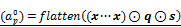 , where flatten(a) vectorizes a matrix a, and (x···x) ∈ RI×J denotes a matrix repeating the vector x J times. In the output layer,
  denotes the value of rj(x,s) defined as
 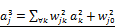 . The hidden layers are expressed as
 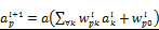 for l=0,1. Here,
  for all p,k,l are coefficients to find by a training process.
Results
We evaluate Tiresias using both real and synthetic datasets. In real datasets, only part of interacting pairs between miRNAs and mRNAs have been discovered by biological experiments. This makes the real datasets inadequate to compute accuracy metrics for any algorithms, for which perfect ground truth is necessary. Thus, our experiments first start with a synthetic dataset, where we generate a number of ground-truth pairs. In such a controlled environment, we evaluate Tiresias with comparison to existing relevant algorithms in terms of precision and recall, and also examine the effects of internal parameters of Tiresias. After getting a sense of the general trend in the performance of Tiresias, we then apply Tiresias to multiple real datasets. In the experiments with real datasets for several diseases, we will see how well Tiresias performs in deciphering the validated interacting pairs, and what kind of new pairs are newly predicted to be interacting.
Synthetic dataset
Experiment environment
We implemented Tiresias using Tensorflow [24]. For the Bayesian optimization, we used an open-source software downloaded from [25]. In order to train, we generated a synthetic dataset of 1000 samples. Each sample of the dataset contains 20 miRNAs and 200 mRNAs. For each mRNA, we randomly selected 10 miRNAs for putative interactions (i.e., qij = 1), and 5 miRNAs among them to regulate the mRNA (i.e., sij = 1) with a random direction (i.e., wij > 0 or wij < 0), biased to down-regulations.6 Thus, we have, in total, 4000 pairs of miRNAs and mRNAs, and 1000 ground truth interactions among 2000 putative interactions.
The expressions of mRNAs were generated following Equation (1) and Equation (2) with xi ~ N(3,1), μj = 10, and  . We tested 4 different magnitudes of the regulation weights |wij|: 0.05, 0.10, 0.15, and 0.2. Note in this setup that the value of Pearson correlation coefficient (PCC) for an interacting pair becomes, on average, the same as the value of the corresponding regulation weight. The optimal value of ρ was chosen to be 0.25. In all experiments that follow, we set N1 = 100, N2 = 10, K = 1, λ1 = 1, and λ2 = 1, unless otherwise stated.
Performance comparison
Figure 5A presents quality measures of recovering interactions between miRNAs and mRNAs for Tiresias, GenMiR++, Elastic Net, and PIMiM.7 For Tiresias, we decided eij as a positive if |eij| > 0.001 and the sign of eij matches the regulation direction that was randomly chosen by our synthetic data generator. The same rule and threshold applied to Elastic Net and PIMiM. For GenMiR++, we declared a positive if its own estimation metric, i.e., β in [12], is > 0.5.
In the figure, it is worth noting that Tiresias achieves a F1 score >0.8 at |wij| ≥ 0.10, which means that in practice, Tiresias can successfully predict regulatory interactions of over a certain strength with a low false positive rate. Meanwhile, other methods show poor performance in the same situations, resulting in F1 scores ranging from 0.2 to 0.6. GenMiR++ is expected to perform better if there exist down-regulations only in the dataset, since it is strictly limited to search down-regulations. The figure should be understood as what GenMiR++ can achieve when applied to the dataset that may contain up-regulations as well. This indicates why we need an algorithm like Tiresias that is designed to consider up-regulations in addition to down-regulations. Elastic Net usually performs poorly unless the regulation effect is significantly strong as can be seen in [26]. PIMiM is reported in [13] to achieve the F1 score of about 0.37. Our experiment confirms the result, showing a similar level of a F1 score. We think that PIMiM may be good for grouping genes, which is its intended purpose, but may not be suitable for predicting miRNA targets.
Effect of the number of samples, miRNAs or mRNAs
Figures 5B, 5C and 5D show the F1 score of Tiresias according to the number of samples, miRNAs, and mRNAs. Increase in the number of samples provides Tiresias with more information, and thus it is always helpful for improving the performance, as one may imagine. In the meantime, as we can see from Equation (2) that the number of miRNAs that we are analyzing at a time is the number of terms that are summed in rj(x,s). Thus, the increase in that number means the level of additive noise gets higher, which results in degradation in performance. Figure 5C shows such an aspect, and suggests that in practice, Tiresias should set a limit for the number of miRNAs to analyze at a time in order to achieve a high F1 score. Note that this is a limitation of all approaches that analyze multi-dimensional data at the same time. One can imagine from Figure 5A that Tiresias would still outperform other competitors in the same situation. However, from Figure 5D, we can see that the performance of Tiresias is less sensitive to the increase in the number of mRNAs than the increase in the number of miRNAs. This is because minimizing the magnitude of c'(x,y) can eventually help minimize the magnitude of 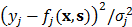 for each j, although affected with more error sources with the increase in the number of mRNAs.
Effect of K
Figure 5E shows how the value of  changes according to K, the number of features extracted from the autoencoder in Figure 2C. As can be seen,
  , the average of c1(x,y) in Equation (12) near convergence, keeps increasing along with K, showing that the expressions of 20 miRNAs and 200 mRNAs can be surprisingly well represented with one single feature (K = 1). Increasing the value of K seems to make training h(x,y) more difficult, since it also increases the number of unknown coefficients of g(x,y).
Effects of λ1 and λ2
Figures 5F and 5G show the variation of  according to λ1 and λ2, the weights for the penalty terms in Equation (10). We can see from the figures that λ1 and λ2 do not significantly affect
  . This is because near the end of training h(x,y), the penalty terms get trivially small so that c'(x,y) is usually dominated by c1(x,y). For this reason, we can omit optimizing the values of λ1 and λ2 by Bayesian optimization, although they are also hyper-parameters.
Breast invasive carcinoma dataset
Experiment environment
In order to test Tiresias on real biological data, we first consider a breast invasive carcinoma dataset (project ID TCGA-BRCA) from the Cancer Genome Atlas (TCGA) portal [17], where 1098 samples of expression data from breast cancer patients are available. Evaluation is done by checking if Tiresias can result in a significant value of eij with a right sign when the i-th miRNA and the j-th mRNA are “truly interacting”. To this end, we built up the true regulation relationship, and their direction and strength from experiment-validated databases, as follows.
The ground truth interactions between miRNAs and mRNAs for breast cancer were checked using the miRTarBase portal [27], which provides experimentally-validated miRNA-target databases. To increase the reliability of the ground truth, we only counted the pairs of miRNAs and mRNAs that are validated more than 3 times by multiple papers, given the lack of high-confidence validated miRNA-target predictions. This resulted in 24 interacting pairs between 19 miRNAs and 19 mRNAs, i.e., I = 19 and J = 19. The names of selected miRNAs and mRNAs are shown in Figure 6C. Note here that the absence of an interaction in miRTarBase for other pairs does not necessarily mean that the pairs are not actually interacting. Some of such pairs may be interacting, but are not yet validated by experiments. This implies that in the experiment, we cannot evaluate the precision and recall of Tiresias, because some none-validated interacting pairs may be counted as false positives. For this reason, we focus here on evaluating how well Tiresias can decipher the 24 validated interacting pairs from the expression dataset by a detection rate, which we define as a ratio of the number of detection to the total number of validated interacting pairs.
(A) Bayesian optimization process, where the utility means the value of the acquisition function by which we can decide the next value of ρ to try, based on the history so far. (B) PCCs for TCGA-BRCA dataset. (C) Heat map of the regulatory network edge matrix e estimated by Tiresias for TCGA-BRCA dataset. A putative interacting pair is marked as ○. Down-regulation (of a negative PCC) and up-regulation (of a positive PCC) are marked as ▽ and △, respectively, for the ground truth interactions. For the pairs whose PCC magnitude is >0.1, the triangle markers get larger, proportional to their PCC magnitude, and they are colored black. (D) Regulation strength and direction. Here, the strength in the vertical axis is the PCC values for validated interacting pairs in case of the ground truth, and the estimated values of eij's in case of Tiresias. In the horizontal axis, (x,y) means the miRNA index x and the mRNA index y in (C). (E)-(F) Detection rate for validated pairs after filtering by PCC values. The “threshold" in the x-axis is such that we decide eij as a detection if |eij| > 'threshold' and the sign of eij matches the sign of its PCC. This figure shows that Tiresias can decipher interacting pairs of miRNAs and mRNAs with a high rate if the regulation strength is over a certain magnitude (e.g., PCC ≥ 0.1). (G)-(H) Normality test. (G) is the Q-Q plot for mRNAs of TCGA breast cancer dataset where different colors represent different mRNAs. (H) is a histogram of (non-scaled) mRNA ERBB3 expressions showing the typical characteristics of TCGA dataset distributions: the left tail is truncated and there exist outliers of a large magnitude. (I) Regression error reduction by switching to a non-linear regulation model. The non-linear regulation model in Figure 4 achieves 12% (on average over mRNAs) less regression error than the linear regulation model in Equation (2).
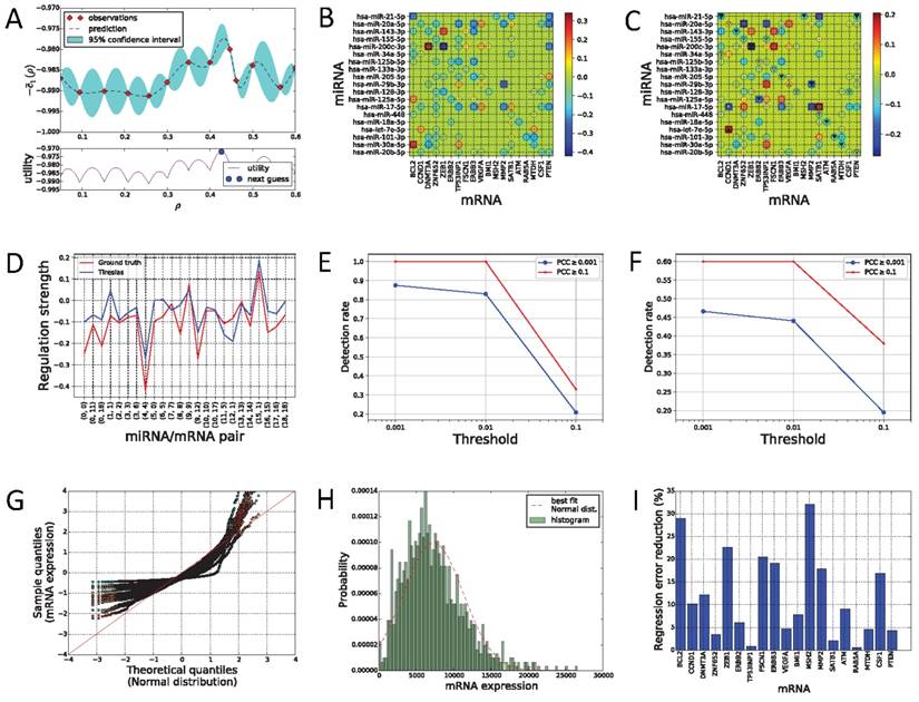
The ground truth directions (up or down) and strengths of regulations were determined based on PCC, a measure of the linear correlation, between an miRNA and an mRNA for the known interacting pairs, as in other literature [28]. However, it should be noted that although the PCC can decide the regulation strength and direction for the validated interacting pairs, the PCC value itself cannot tell us which pairs are interacting, since non-interacting pairs may also show a significant value of PCC. As shown in Figure 6B, most putative interactions indeed have a non-negligible value of PCC. We will see that Tiresias, which finds interaction relationships based on e, not PCC, can filter out such putative interactions that have significant PCCs.
The putative interaction matrix q was made by sequence-based prediction results, downloaded from TargetScan [2] version 7.1, which includes non-canonical sites. The optimal value of ρ was determined to be 0.446 by Bayesian optimization as shown in Figure 6A.
Estimated regulatory network
The regulatory network edge matrix e in Equation (13), estimated by Tiresias, is expressed as a heat map in Figure 6C, where a positive  indicates the up-regulation and a negative eij is the down-regulation between the i-th miRNA and the j-th mRNA. The results for the validated pairs are summarized in Figure 6D separately. We can see from the figures that Tiresias can predict most of the validated interacting pairs with the right direction—negative regulation weights for negative PCC values and positive regulation weights for positive PCC values. We also note that the magnitude of eij is proportional to the magnitude of PCC in most cases. Exceptions are three pairs, (hsa-miR-34a-5p, BCL2), (hsa-miR-125b-5p, ERBB2), and (hsa-miR-20b-5p, PTEN). We think that those pairs are not predicted by Tiresias because their PCCs are too small, and there exist other miRNAs that have a larger PCC for the mRNAs. In such outlier cases, these subtle interactive tendencies, latent in their expression levels, may have been outweighed by more functionally meaningful interactions, as learned by Tiresias.
Figure 6E that shows Tiresias's detection rate for the validated pairs, after filtering by PCC values in a way that the ground-truth interaction is assumed if PCC ≥ 0.1 or PCC ≥ 0.001. We can see that Tiresias's detection performance is naturally dependent on the regulation strength, i.e., easier to detect if a regulation is strong. However, we can also see that the detection rate of Tiresias is still high enough (>0.8) even if we assume that true regulation relationship may result in a small value of PCC (PCC ≥ 0.001). Figure 6F also shows the detection rate of Tiresias when we increment the numbers of miRNAs and mRNAs under consideration. For this experiment, the candidates of ground-truth interaction pairs before filtering by PCC values are selected if only one paper is reported interacting in miRTarBase, which leads to 119 interacting pairs between 60 miRNAs and 99 mRNAs. As we can see in Figure 5C, the increase in the number of miRNAs means a higher noise level and thus lower performance, which is naturally unavoidable. Thus, we can see from the figure that Tiresias's detection rate is lower than in Figure 6E. Although Tiresias can still achieve ~0.6 detection rate in this case, this suggests us to use Tiresias with a practical limit in the number of miRNAs at a time to build high confidence. We may consider dividing the dataset into multiple ones, each of which contains partial lists of miRNAs, and applying Tiresias to each smaller dataset. By changing the way of separating the dataset, and iterating detection on each partial dataset, we can still see the joint effect among miRNAs. From Figure 6C, we can also see that since PCCs are usually small even for the ground truth pairs (non-black triangle markers in Figure 6C), corresponding values of |eij| are mostly small and thus the detection threshold of Tiresias must be set small enough (<0.01).
Normality test
We test the normality of mRNAs expressions for the TCGA breast cancer dataset, since we began with assuming that yj for any j is normally distributed as in Equation (1). Figure 6G shows a Q-Q plot for distributions of mRNA expressions versus the Normal distribution, where each color of dots corresponds to one kind of an mRNA. The Q-Q plot is a plot of the quantiles of one dataset against the quantiles of the other dataset, providing a graphical method for comparing probability distributions of two datasets.8 We can see that TCGA dataset deviates from the Normal distribution especially where a sample expression is far from a mean (quantile 0). Indeed, the typical shape of an mRNA distribution from TCGA dataset looks like Figure 6H, which is rather more similar to the truncated normal distribution with outliers of a large magnitude. D'Agostino-Pearson omnibus tests presented in Section S2 of Supplementary material confirm that each mRNA is not normally distributed. However, since Tiresias is a kind of a regression method minimizing the mean squared error between f(x,s) and y, it can be considerably robust to violation of normality, as long as the sample size is reasonably large. We think that this robustness contributed to the high detection rates of Tiresias as in Figure 6E.
Non-linear regulation
Figure 6I shows regression error reduction for each mRNA by switching from the linear regulation model in Equation (2) to the non-linear regulation model in Figure 4. Here, the regression error for yj is defined as:
, (15)
in which the superscript (m) over a value means that the value comes from the m-th data sample, as before. We can see that fj(x,s) with the non-linear regulation model fits significantly better to the real data yj in most cases than fj(x,s) with the linear model. On average, the regression error of the non-linear model is 12% smaller than that of the linear model in our experiments. While the linear regulation model considered in existing work, including GenMiR++, Elastic Net, and PIMiM, is intuitive and useful to figure out individual miRNA's strength on regulation, the non-linear model can be used in situations where more accurate regression is required to predict the exact regulation effect for a group of miRNAs. Tiresias can provide such extensibility by easily switching between linearity and non-linearity.
Other real datasets: TCGA-LUAD and TCGA-UCEC
We also applied Tiresias to other real datasets from TCGA, whose project IDs in TCGA site are TCGA-LUAD (Lung Adenocarcinoma), and TCGA-UCEC (Uterine Corpus Endometrial Carcinoma). The TCGA-LUAD dataset has 585 samples, and the TCGA-UCEC dataset consists of 560 samples. The validated interacting pairs were again checked from the miRTarBase portal, but this time we took all pairs into account that were reported interacting at least once in literature, due to their lower popularity. From Figure 5B, performance of Tiresias is expected to be lower than in TCGA-BRCA, since the number of samples available is much lower. Other factors of experimental setup are the same as before, unless otherwise stated.
Lung Adenocarcinoma
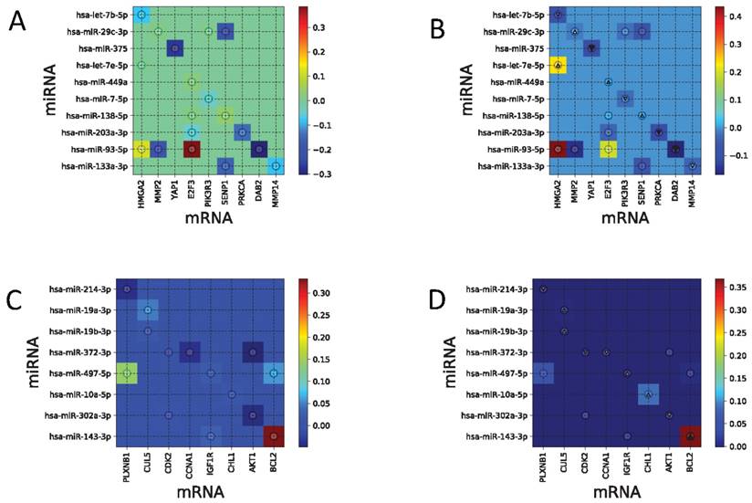
Figures 7A and 7B shows PCCs for the TCGA-LUAD dataset and the regulatory network edge matrix e estimated by Tiresias, where the value of ρ was chosen to be 0.15. The TCGA-LUAD dataset has characteristics that all the putative interacting pairs have non-zero PCCs, and validated interacting pairs are mostly of small PCC. As we have observed in the previous experiments, Tiresias may fail to detect the interacting pairs if their true regulation strength is too small. In this case, Tiresias missed two pairs in detection, which are (hsa-miR-449a, E2F3) and (hsa-miR-138-5p, SENP1). However, note that (hsa-let-7e-5p, HMGA2) and (hsa-miR-7-5p, PK3R3) were detected with significant strength, although their PCCs are negligibly small. Those pairs cannot be detected when we try to find them by using PCC values higher than a certain threshold.
(A) PCCs for TCGA-LUAD data set. (B) Regulatory network edge matrix e for TCGA-LUAD, estimated by Tiresias. Note that (hsa-let-7e-5p, HMGA2) and (hsa-miR-7-5p, PK3R3) are detected with significant strength, although their PCCs are negligibly small. (C) PCCs for TCGA-UCEC data set. (D) Regulatory network edge matrix e for TCGA-UCEC, estimated by Tiresias. Note that that Tiresias can detect (hsa-miR-10a-5p, CHL1) even though its PCC is almost zero, and suppress putative interactions with relatively large PCC like (hsa-miR-372-3p, AKT1) and (hsa-miR-497-5p, BCL2).
Uterine Corpus Endometrial Carcinoma
Figures 7C and 7D shows PCCs for the TCGA-UCEC dataset and the regulatory network edge matrix e estimated by Tiresias with ρ = 0.03. What we observed from the TCGA-UCEC dataset is that only one validated interacting pair has a significant value of PCC, and others have almost zero PCC. So as in the TCGA-LUAD case, Tiresias misses several validated pairs in detection. However, note that they are the ones that are also difficult to detect from the PCC-based threshold test. We also note that Tiresias can detect (hsa-miR-10a-5p, CHL1) even though its PCC is almost zero, and suppressed putative interactions with relatively large PCC like (hsa-miR-372-3p, AKT1) and (hsa-miR-497-5p, BCL2).
Discussion
In this paper, we proposed Tiresias, a new computational method based on ANNs for predicting which mRNAs are targeted by which miRNAs. Tiresias separately considers the miRNA target estimation and the regulation weight estimation by building an ANN for each problem. However, in the training phase, Tiresias combines them together as a single two-stage ANN, which enables us to associate the two problems and solve them simultaneously.
Our prediction is context-specific, i.e., takes into account what kind of diseased state the cell is in and incorporates expression-level data in addition to sequence-based prediction data. Experimental results showed that Tiresias performs better than existing computational methods such as GenMiR++, Elastic Net, and PIMiM, achieving an F1 score of >0.8 for a certain level of regulation strength. For the TCGA breast cancer dataset, Tiresias showed a true positive rate of up to 82% in recovering the ground truth regulatory interactions between miRNAs and mRNAs, even when we assume that the regulations may lead to small PCCs.
Tiresias predicted new interacting pairs in Figures 6C, 7B, and 7D (non-zero eij for putative interactions). Since Tiresias is expected to have a low false positive rate from Figure 5A, those may be considered suitable candidates for future validation via biological experiments. The full list of miRNA-mRNA pairs that are predicted to be interacting by Tiresias can be found in the Supplementary material.
In order to further improve the F1 score, we can also consider incorporating other regulatory factors such as transcription factors into our model as an input to the miRNA target estimation network g(x,y), in addition to x and y. Then, the autoencoder part should be able to extract more meaningful features and thus improve prediction performance. Further, we can conceive of adding Protein-Protein Interaction (PPI) network information to our model as done in [13] and expect this to be increasingly useful as such PPI network information becomes denser. We can incorporate this into our model by adding a further penalty function to Equation (10), which will penalize a solution that puts mRNAs associated with interacting proteins in different modules since interacting proteins are more likely to be co-regulated by the same miRNAs [31, 32].
Note that although Tiresias is an explanatory model that analyzes the given dataset, we can also make use of the trained Tiresias as an mRNA expression level predictor for given miRNA expressions. With the capability to extend into a non-linear regulation model, Tiresias can achieve a highly accurate prediction to the level of mRNA expression.
We have currently used TargetScan for determining the necessary conditions for miRNA-mRNA interactions. This can be replaced with other sequence-based methods that are being actively developed for predicting such putative interactions, including our recent work [7], which is able to look for non-canonical sequence matches as well. A more accurate determination of such priors will further improve the performance of Tiresias.
We have used stochastic gradient descent for training, iterating over the TCGA samples 100 times, at which point, convergence is reached. On a Dell PowerEdge R320 server of 12 Intel Xeon processors, it takes Tiresias ~10 min to complete training for a given value of ρ, including feature extraction by an autoencoder. We then use Bayesian optimization to find an optimal value of ρ, which in all our experiments, happens within 10 iterations.
Abbreviations
miRNA: microRNA; mRNA: messenger RNA; ANN: artificial neural network; PAR-CLIP: photoactivatable ribonucleoside-enhanced crosslinking and immunoprecipitation; HITS-CLIP: high-throughput sequencing of RNA isolated by crosslinking immunoprecipitation; PCC: Pearson correlation coefficient; EM: expectation maximization; TCGA: the Cancer Genome Atlas; pdf: probability density function; MSE: mean squared error; BRCA: breast invasive carcinoma; LUAD: lung adenocarcinoma; UCEC: uterine corpus endometrial carcinoma.
Supplementary Material
Supplementary figures and tables.
Competing Interests
The authors have declared that no competing interest exists.
References
1. Griffiths-Jones S, Grocock RJ, Dongen S, Bateman A, Enright AJ. mirbase: microrna sequences, targets and gene nomenclature. Nucleic Acids Res. 2006;34:D140-D144
2. Agarwal V, Bell GW, Nam J-W, Bartel DP. Predicting effective microrna target sites in mammalian mrnas. eLife. 2015;4:e05005
3. Betel D, Koppal A, Agius P, Sander C, Leslie C. Comprehensive modeling of microrna targets predicts functional non-conserved and non-canonical sites. Genome Biol. 2010;11(8):R90
4. Khorshid M, Hausser J, Zavolan M, Nimwegen E. A biophysical mirna-mrna interaction model infers canonical and noncanonical targets. Nat methods. 2013;10(3):253-255
5. Asirvatham AJ, Gregorie CJ, Hu Z, Magner WJ, Tomasi TB. Microrna targets in immune genes and the dicer/argonaute and are machinery components. Mol Immunol. 2008;45(7):1995-2006
6. Ghoshal A, Shankar R, Bagchi S, Grama A, Chaterji S. Microrna target prediction using thermodynamic and sequence curves. BMC Genomics. 2015;16:999
7. Ghoshal A, Grama A, Bagchi S, Chaterji S. An ensemble svm model for the accurate prediction of non-canonical microrna targets. ACM BCB. 2015:403-412
8. Fulci V, Colombo T, Chiaretti S, Messina M, Citarella F. et al. Characterization of b- and t-lineage acute lymphoblastic leukemia by integrated analysis of microrna and mrna expression profiles. Genes Chromosomes Cancer. 2009;48(12):1069-1082
9. Lu Y, Zhou Y, Qu W, Deng M, Zhang C. A lasso regression model for the construction of microrna-target regulatory networks. Bioinformatics. 2011;27(17):2406-2413
10. Beck D, Ayers S, Wen J, Brandl MB, Pham TD. et al. Integrative analysis of next generation sequencing for small non-coding rnas and transcriptional regulation in myelodysplastic syndromes. BMC Med Genomics. 2011;4(1):19
11. Huang JC, Morris QD, Frey BJ. Detecting MicroRNA Targets by Linking Sequence, MicroRNA and Gene Expression Data, RECOMB. 2006; 114-129.
12. Huang JC, Babak T, Corson TW, Chua G, Khan S. et al. Using expression profiling data to identify human microrna targets. Nat Methods. 2007;4(12):1045-1049
13. Le H-S, Bar-Joseph Z. Integrating sequence, expression and interaction data to determine condition-specific mirna regulation. Bioinformatics. 2013;29(13):i89-i97
14. Vasudevan S. Posttranscriptional upregulation by micrornas. Wiley Interdiscip Rev RNA. 2012;3(3):311-330
15. Shu J, Xia Z, Li L, Liang ET, Slipek N. et al. Dose-dependent differential mrna target selection and regulation by let-7a-7f and mir-17-92 cluster micrornas. RNA Biology. 2012;9(10):1275-1287
16. Lai X, Wolkenhauer O, Vera J. Understanding microrna-mediated gene regulatory networks through mathematical modelling. Nucleic Acids Res. 2016;44(13):6019-6035
17. The Cancer Genome Atlas. http://cancergenome.nih.gov/
18. Law of large numbers. https://en.wikipedia.org/wiki/Law_of_large_numbers
19. Dayan P, Hinton GE, Neal RN, Zemel RS. The Helmholtz machine. Neural Computation. 1995;7:889-904
20. Ng A. Sparse autoencoder. https://web.stanford.edu/class/cs294a/sparseAutoencoder.pdf
21. Schmidhuber J. Deep learning in neural networks: An overview. Neural Networks. 2015;61:85-117
22. Brochu E, Cora VM, Freitas N. A tutorial on bayesian optimization of expensive cost functions, with application to active user modeling and hierarchical reinforcement learning. CoRR. 2010 arXiv:1012.2599
23. Shmueli G. To explain or to predict? Statist Sci. 2010;25(3):289-310
24. TensorFlow: A system for large-scale machine learning. https://www.tensorflow.org
25. Bayesian Optimization. https://github.com/fmfn/BayesianOptimization
26. Sass S, Pitea A, Unger K, Hess J, Mueller NS, Theis FJ. Microrna-target network inference and local network enrichment analysis identify two microrna clusters with distinct functions in head and neck squamous cell carcinoma. Int J Mol Sci. 2015;16(12):30204-30222
27. miRTarBase. The experimentally validated miRNA-target interactions database. http://mirtarbase.mbc.nctu.edu.tw
28. Wang YP, Li KB. Correlation of expression profiles between micrornas and mrna targets using nci-60 data. BMC Genomics. 2009;10:218
29. Q-Q plot. https://en.wikipedia.org/wiki/Q-Q_plot
30. Yan X, Su XG. Linear Regression Analysis: Theory and Computing. River Edge, NJ, USA: World Scientific Publishing Co Inc. 2009
31. Liang H, Li WH. Microrna regulation of human protein-protein interaction network. RNA. 2007;13(9):1402-1408
32. Hsu CW, Juan HF, Huang HC. Characterization of microrna-regulated protein-protein interaction network. Proteomics. 2008;8(10):1975-1979
Footnotes
Tiresias is a Greek character who was famous for his ability to see precisely into the future. He achieved this without needing to see into all the details of the present. Similarly, our model is unaware of the exact interaction priors but is able to infer them from the data and generate new predictions for miRNA-mRNA interactions.
Later, we will discuss how to extend this to non-linear regulation models.
Although this network does not currently contain any activation function like a sigmoid function, we stick to calling it an ANN in case we replace rj(x,s) with a multi-layer ANN to study non-linear regulation effects.
The features can also be extracted by using multi-layer ANNs, i.e., deeper ANNs in order to reflect more complex non-linearity.
Technically, λ1 and λ2 are also hyper-parameters, but we have found by experiments that they are not critical compared to ρ (see Figures 5F and 5G). Thus, we can simply set them all to 1, and focus on tuning ρ.
Regarding the rareness of up-regulations, the probabilities of generating up-regulation and down-regulation are set to 0.1 and 0.9, respectively.
Note that GenMiR++ and PIMiM were originally designed to find down-regulations only. For this experiment, we modified PIMiM to detect up-regulations as well. However, GenMiR++ was used as is, since this method is inherently restricted to down-regulations by their modeling. Protein interaction matrix required for PIMiM was assumed to be an all-zero matrix, since it is usually very sparse.
A formal definition of the Q-Q plot can be found at [29].
Author contact
![]() Corresponding author: schaterjiorg
Corresponding author: schaterjiorg